IT评测·应用市场-qidao123.com技术社区

标题: PyTorch与TensorFlow模子全方位解析：保存、加载与结构可视化 [打印本页]

作者: 王柳 时间: 5 天前
标题: PyTorch与TensorFlow模子全方位解析：保存、加载与结构可视化
目次

前言
一、保存整个模子
二、pytorch模子的加载
2.1 只保存的模子参数的加载方式：
2.2 保存结构和参数的模子加载
三、pytorch模子网络结构的查看
3.1 print
3.2 summary
3.3 netron
3.3.1 解决方法1
3.3.2 解决方法2
3.4 TensorboardX
四、tensorflow 框架的线性回归
4.1 tensorflow模子的定义
4.1.1 tf.keras.Sequential
4.1.2 tf.keras.Sequential()另一种方式
4.1.3 就是写一个类重写实现网络的搭建
4.1.4 tensorflow中最常用的
4.2 tensorflow模子的保存
4.2.1 保存为 .h5
4.2.2 只保存参数
4.3 tensorflow模子的加载
4.3.1 模子加载针对方式1
4.3.2 加载只保存参数，包括权重w及偏置b
4.4 tensorflow模子网络结构的查看
4.4.1 summary() 模子搭建好就有summary()
4.4.2 使用netron
4.4.3 最经典的 tensorboard 方法
总结

前言

书接上文
PyTorch 线性回归详解：模子定义、保存、加载与网络结构-CSDN博客本文全面阐述了PyTorch框架下线性回归的实现过程，涵盖了模子定义的不同方式（如nn.Sequential、nn.ModuleList等）、模子保存方法（torch.save()），以及模子加载和网络结构查看。结合具体代码示例，旨在帮助读者深入理解并把握PyTorch在解决线性回归问题中的应用。

https://blog.csdn.net/qq_58364361/article/details/147329215?spm=1011.2415.3001.10575&sharefrom=mp_manage_link

一、保存整个模子

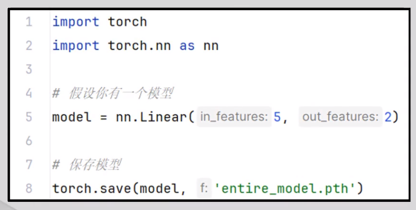
保存：要保存整个模子，包括其结构和参数，可以使用torch.save()函数保存整个模子。

将整个模子保存到名为"entire_model.pth"的文件中。但是要注意，保存整个模子大概会占用更多的磁盘空间，并且不如保存状态字典机动，由于状态字典可以与不同的模子结构兼容。

import torch
import numpy as np
# 1. 数据准备
# 定义原始数据，包含x和y值
data = [[-0.5, 7.7], [1.8, 98.5], [0.9, 57.8],
[0.4, 39.2], [-1.4, -15.7],
[-1.4, -37.3], [-1.8, -49.1],
[1.5, 75.6], [0.4, 34.0],
[0.8, 62.3]]
# 将数据转换为NumPy数组，方便后续处理
data = np.array(data)
# 从NumPy数组中提取x和y数据
x_data = data[:, 0] # 所有行的第0列，即x值
y_data = data[:, 1] # 所有行的第1列，即y值
# 2. 数据转换为Tensor
# 将NumPy数组转换为PyTorch张量，这是使用PyTorch进行计算的基础
x_train = torch.tensor(x_data, dtype=torch.float32) # 将x数据转换为float32类型的张量
y_train = torch.tensor(y_data, dtype=torch.float32) # 将y数据转换为float32类型的张量
# 3. 使用DataLoader加载数据
# 导入DataLoader和TensorDataset
from torch.utils.data import DataLoader, TensorDataset
# 将x_train和y_train组合成一个数据集
dataset = TensorDataset(x_train, y_train) # 创建一个TensorDataset，将x和y数据配对
# 使用DataLoader创建数据加载器，用于批量处理数据
dataloader = DataLoader(dataset, batch_size=2, shuffle=False) # batch_size=2表示每次加载2个样本，shuffle=False表示不打乱数据顺序
# 4. 定义模型
import torch.nn as nn # 导入torch.nn模块，通常简写为nn，包含神经网络相关的类和函数
# 定义线性回归模型
class LinearModel(nn.Module): # 继承nn.Module，这是所有神经网络模块的基类
# 构造函数，用于初始化模型
def __init__(self):
super(LinearModel, self).__init__() # 调用父类的构造函数
# 定义一个线性层，输入维度为1，输出维度为1
self.layers = nn.Linear(1, 1) # 创建一个线性层，用于学习线性关系
# 前向传播函数，定义模型的计算过程
def forward(self, x):
# 将输入x通过线性层
x = self.layers(x) # 将输入数据通过线性层进行计算
return x # 返回计算结果
# 5. 初始化模型
# 创建模型实例
model = LinearModel() # 实例化线性回归模型
# 6. 定义损失函数
# 使用均方误差作为损失函数
criterion = nn.MSELoss() # 创建MSELoss实例，用于计算损失
# 7. 定义优化器
# 使用随机梯度下降算法作为优化器
optimizer = torch.optim.SGD(model.parameters(), lr=0.01) # 创建SGD优化器，用于更新模型参数, lr是学习率
# 8. 训练模型
# 设置迭代次数
epoches = 500 # 设置迭代次数
# 循环迭代训练模型
for n in range(1, epoches + 1): # 迭代epoches次
epoch_loss = 0 # 初始化epoch损失
# 遍历dataloader，获取每个batch的数据
for batch_x, batch_y in dataloader: # 遍历dataloader，每次返回一个batch的x和y数据
# 增加x_batch的维度，以匹配线性层的输入维度
x_batch_add_dim = batch_x.unsqueeze(1) # 在第1维增加一个维度，将x_batch从[batch_size]变为[batch_size, 1]
# 使用模型进行预测
y_pre = model(x_batch_add_dim) # 将x_batch输入模型，得到预测值
# 计算损失
batch_loss = criterion(y_pre.squeeze(1), batch_y) # 计算预测值和真实值之间的均方误差, squeeze(1) 移除维度为1的维度
# 梯度更新
optimizer.zero_grad() # 清空优化器中的梯度，避免累积
# 计算损失函数对模型参数的梯度
batch_loss.backward() # 反向传播，计算梯度
# 根据优化算法更新参数
optimizer.step() # 使用优化器更新模型参数
epoch_loss = epoch_loss + batch_loss # 累加每个batch的损失
avg_loss = epoch_loss / (len(dataloader)) # 计算平均损失
# 打印训练信息
if n % 100 == 0 or n == 1: # 每100次迭代打印一次信息
print(model) # 打印模型结构
torch.save(model, f'model_{n}.pth') #保存模型
print(f"epoches:{n},loss:{avg_loss}") # 打印迭代次数和损失值

复制代码

二、pytorch模子的加载

模子的保存有两种方式，模子的加载也有两种方式
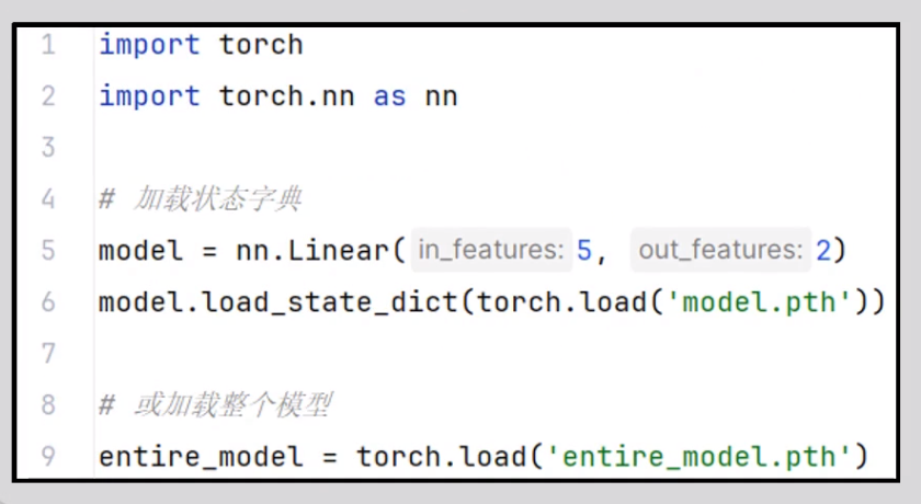
加载：
要加载保存的模子，使用torch.load()函数

2.1 只保存的模子参数的加载方式：

加载模子必要3步骤：
步骤1：必要模子结构(保存时搭建的模子)
步骤2：使用torch.load("model.pth")加载模子参数
步骤3：:实例化模子（model）使用model.load_state_dict(torch.load("model.pth"))将model和参数结合起来

import torch.nn as nn
import torch
import numpy as np
# 示例数据
data = [[-0.5, 7.7], [1.8, 98.5], [0.9, 57.8], [0.4, 39.2], [-1.4, -15.7], [-1.4, -37.3], [-1.8, -49.1], [1.5, 75.6],
[0.4, 34.0], [0.8, 62.3]]
data = np.array(data)
x_data = data[:, 0] # 获取 x 数据
y_data = data[:, 1] # 获取 y 数据
x_train = torch.tensor(x_data, dtype=torch.float32) # 将 x 数据转换为 PyTorch 张量
y_train = torch.tensor(y_data, dtype=torch.float32) # 将 y 数据转换为 PyTorch 张量
from torch.utils.data import DataLoader, TensorDataset
dataset = TensorDataset(x_train, y_train) # 创建 TensorDataset
dataloader = DataLoader(dataset, batch_size=2, shuffle=False) # 创建 DataLoader
import torch.nn as nn
class LinearModel(nn.Module):
"""
线性模型类
"""
def __init__(self):
"""
初始化线性模型
"""
super(
LinearModel,
self,
).__init__()
# 定义一个线性层
self.layers = nn.Linear(1, 1)
def forward(
self,
x
):
"""
前向传播函数
:param x: 输入张量
:return: 输出张量
"""
x = self.layers(x) # 通过线性层
return x
model = LinearModel() # 实例化线性模型
model.load_state_dict(torch.load("model_1.pth")) # 加载模型参数
model.eval() # 设置为评估模式
x_test = torch.tensor([[-0.5]], dtype=torch.float32) # 创建测试数据
with torch.no_grad(): # 禁用梯度计算
y_pre = model(x_test) # 进行预测
print(y_pre) # 打印预测结果

复制代码

2.2 保存结构和参数的模子加载

加载模子必要2步骤：
步骤1：必要模子结构
步骤2：使用torch.load("entire_model.pth")加载模子

import torch
import numpy as np
# 准备数据：输入特征和对应的目标值
data = [[-0.5, 7.7], [1.8, 98.5], [0.9, 57.8], [0.4, 39.2], [-1.4, -15.7], [-1.4, -37.3], [-1.8, -49.1], [1.5, 75.6],
[0.4, 34.0], [0.8, 62.3]]
data = np.array(data)
# 提取输入特征 (x) 和目标值 (y)
x_data = data[:, 0]
y_data = data[:, 1]
# 将数据转换为 PyTorch 张量，并指定数据类型为 float32
x_train = torch.tensor(x_data, dtype=torch.float32)
y_train = torch.tensor(y_data, dtype=torch.float32)
# 导入 DataLoader 和 TensorDataset
from torch.utils.data import DataLoader, TensorDataset
# 创建 TensorDataset，将 x_train 和 y_train 组合成数据集
dataset = TensorDataset(x_train, y_train)
# 创建 DataLoader，用于批量加载数据
dataloader = DataLoader(dataset, batch_size=2, shuffle=False)
import torch.nn as nn
# 定义线性模型类
class LinearModel(nn.Module):
def __init__(self):
super(
LinearModel,
self,
).__init__()
# 定义一个线性层，输入维度为 1，输出维度为 1
self.layers = nn.Linear(1, 1)
def forward(
self,
x
):
# 定义前向传播过程
x = self.layers(x)
return x
# 加载预训练的模型
model = torch.load("model_1.pth")
# 将模型设置为评估模式，禁用 dropout 等
model.eval()
# 创建一个测试数据
x_test = torch.tensor([[-0.5]], dtype=torch.float32)
# 在无梯度计算的环境下进行预测
with torch.no_grad():
# 使用加载的模型进行预测
y_pre = model(x_test)
# 打印预测结果
print(y_pre)

复制代码

三、pytorch模子网络结构的查看

3.1 print

print(model) 能打印出网络结构，不能检测模子搭建是否精确
print(model) 仅打印模子结构。

import torch.nn as nn # 导入神经网络模块
import torch # 导入 torch
import numpy as np # 导入 numpy
# 定义数据集，包含输入和输出
data = [[-0.5, 7.7], [1.8, 98.5], [0.9, 57.8], [0.4, 39.2], [-1.4, -15.7], [-1.4, -37.3], [-1.8, -49.1], [1.5, 75.6],
[0.4, 34.0], [0.8, 62.3]]
data = np.array(data) # 将数据转换为 numpy 数组
x_data = data[:, 0] # 获取输入数据
y_data = data[:, 1] # 获取输出数据
x_train = torch.tensor(x_data, dtype=torch.float32) # 将输入数据转换为 tensor
y_train = torch.tensor(y_data, dtype=torch.float32) # 将输出数据转换为 tensor
from torch.utils.data import DataLoader, TensorDataset # 导入 DataLoader 和 TensorDataset
dataset = TensorDataset(x_train, y_train) # 将输入和输出数据组合成 dataset
dataloader = DataLoader(dataset, batch_size=2, shuffle=False) # 创建 dataloader，用于批量加载数据
import torch.nn as nn # 导入神经网络模块
# 定义线性模型
class LinearModel(nn.Module):
def __init__(self):
super(
LinearModel,
self,
).__init__() # 调用父类构造函数
self.layers = nn.Linear(1, 1) # 定义一个线性层，输入维度为 1，输出维度为 1
self.layers1 = nn.Linear(2, 2) # 定义一个线性层，输入维度为 2，输出维度为 2
def forward(
self,
x
): # 定义前向传播函数
x = self.layers(x) # 通过第一个线性层
x = self.layers1(x) # 通过第二个线性层
return x # 返回输出
model = LinearModel() # 实例化模型
print(model) # 打印模型结构

复制代码

3.2 summary

先安装 pip install torchsummary
torchsummary 主要用于查看模子结构并且检测网络是否搭建精确，不精确就报错

import torch.nn as nn # 导入神经网络模块
import torch # 导入torch
import numpy as np # 导入numpy
# 准备数据
data = [[-0.5, 7.7], [1.8, 98.5], [0.9, 57.8], [0.4, 39.2], [-1.4, -15.7], [-1.4, -37.3], [-1.8, -49.1], [1.5, 75.6],
[0.4, 34.0], [0.8, 62.3]]
data = np.array(data) # 转换为numpy数组
x_data = data[:, 0] # 获取x数据
y_data = data[:, 1] # 获取y数据
x_train = torch.tensor(x_data, dtype=torch.float32) # 转换为torch张量
y_train = torch.tensor(y_data, dtype=torch.float32) # 转换为torch张量
from torch.utils.data import DataLoader, TensorDataset # 导入DataLoader和TensorDataset
dataset = TensorDataset(x_train, y_train) # 创建数据集
dataloader = DataLoader(dataset, batch_size=2, shuffle=False) # 创建数据加载器
import torch.nn as nn # 导入神经网络模块
# 定义线性模型
class LinearModel(nn.Module):
def __init__(self):
super(
LinearModel,
self,
).__init__() # 调用父类初始化方法
self.layers = nn.Linear(1, 2) # 定义线性层1，输入维度1，输出维度2
self.layers1 = nn.Linear(2, 5) # 定义线性层2，输入维度2，输出维度5
def forward(
self,
x
): # 定义前向传播函数
x = self.layers(x) # 通过线性层1
x = self.layers1(x) # 通过线性层2
return x # 返回输出
model = LinearModel() # 实例化模型
from torchsummary import summary # 导入summary
summary(
model,
input_size=(1,), # 输入尺寸
device="cpu" # 设备
)

复制代码

3.3 netron

pip install --upgrade netron
netron
pycharm 终端下输入 pip install netron -i Simple Index
下载好后，在终端下输入 netron，在浏览器上输入 http://localhost:8080 即可
netron 用于模子文件的可视化，
问题：netron对pytorch支持欠好，层和层之间没有连线
3.3.1 解决方法1

什么是 JIT？
起首要知道 JIT 是一种概念，全称是 Just In Time Compilation，中文译为「即时编译」，是一种程序优化的方法
将模子保存为脚本文件分两步
step1,先转化为脚本模子
script_model=torch.jit.script(model)
step2保存为文件
torch.jit.save(script_model,"script_model.pth")
使用netron打开有连线了

import torch.nn as nn # 导入神经网络模块
import torch # 导入torch
import numpy as np # 导入numpy
# 准备数据
data = [[-0.5, 7.7], [1.8, 98.5], [0.9, 57.8], [0.4, 39.2], [-1.4, -15.7], [-1.4, -37.3], [-1.8, -49.1], [1.5, 75.6],
[0.4, 34.0], [0.8, 62.3]]
data = np.array(data) # 转换为numpy数组
x_data = data[:, 0] # 获取x数据
y_data = data[:, 1] # 获取y数据
x_train = torch.tensor(x_data, dtype=torch.float32) # 转换为torch张量
y_train = torch.tensor(y_data, dtype=torch.float32) # 转换为torch张量
print(x_train) # 打印x_train
import torch.nn as nn # 再次导入神经网络模块
criterion = nn.MSELoss() # 定义均方误差损失函数
# 定义线性模型
class LinearModel(nn.Module):
def __init__(self):
super(
LinearModel,
self,
).__init__() # 调用父类初始化方法
self.layers = nn.Linear(1, 1) # 定义线性层1，输入维度1，输出维度1
self.layers1 = nn.Linear(1, 2) # 定义线性层2，输入维度1，输出维度2
def forward(
self,
x
): # 定义前向传播函数
x = self.layers(x) # 通过线性层1
x = self.layers1(x) # 通过线性层2
return x # 返回输出
model = LinearModel() # 实例化模型
script_model = torch.jit.script(model) # 将模型转换为 TorchScript
torch.jit.save(script_model, 'script_model.pth') # 保存 TorchScript 模型

复制代码

3.3.2 解决方法2

转成ONNX保存，ONNX(Open Neural Network Exchange)是一个开放的深度学习模子交换格式，它答应在不同的深度学习框架之间共享、迁徙和使用模子。ONNX的目标是提供一个通用的中间表现，使得各种深度学习框架(如pytorch tensorflow MXNeE等)之间能够更轻松交换模子，并且能够在不同框架之间进行模子的部署和推理。
转化为ONNX模子，假如不能运行就安装onnx
安装命令 pip install onnx -i Simple Index

import torch.nn as nn # 导入神经网络模块
import torch # 导入torch
import numpy as np # 导入numpy
# 准备数据，这里是一些二维数据点
data = [[-0.5, 7.7], [1.8, 98.5], [0.9, 57.8], [0.4, 39.2], [-1.4, -15.7], [-1.4, -37.3], [-1.8, -49.1], [1.5, 75.6],
[0.4, 34.0], [0.8, 62.3]]
data = np.array(data) # 将数据转换为numpy数组，方便后续处理
x_data = data[:, 0] # 从数据中提取x坐标
y_data = data[:, 1] # 从数据中提取y坐标
x_train = torch.tensor(x_data, dtype=torch.float32) # 将x坐标转换为torch张量，并指定数据类型为float32
y_train = torch.tensor(y_data, dtype=torch.float32) # 将y坐标转换为torch张量，并指定数据类型为float32
print(x_train) # 打印x_train，用于调试
import torch.nn as nn # 再次导入神经网络模块，虽然已经导入过，但为了代码完整性保留
criterion = nn.MSELoss() # 定义均方误差损失函数，用于衡量模型预测值和真实值之间的差距
# 定义一个线性模型类，继承自nn.Module
class LinearModel(nn.Module):
def __init__(self):
# 调用父类的初始化方法
super(
LinearModel,
self,
).__init__()
# 定义一个线性层，输入维度为1，输出维度为1
self.layers = nn.Linear(1, 1)
# 定义一个线性层，输入维度为1，输出维度为2
self.layers1 = nn.Linear(1, 2)
# 定义一个线性层，输入维度为2，输出维度为2
self.layers2 = nn.Linear(2, 2)
def forward(
self,
x
):
# 定义模型的前向传播过程
x = self.layers(x) # 将输入x通过第一个线性层
x = self.layers1(x) # 将第一个线性层的输出通过第二个线性层
x = self.layers2(x) # 将第二个线性层的输出通过第三个线性层
return x # 返回模型的输出
model = LinearModel() # 实例化线性模型
torch.onnx.export(
model, # 要导出的模型
torch.rand(1, 1), # 模型的输入，这里使用一个随机张量
"model1.onnx" # 导出的onnx模型的文件名
)

复制代码

3.4 TensorboardX

TensorboardX 这个工具使得 pytorch 框架也可以使用到 Tensorboard 的便捷功能。
安装：
pip install TensorboardX -i Simple Index
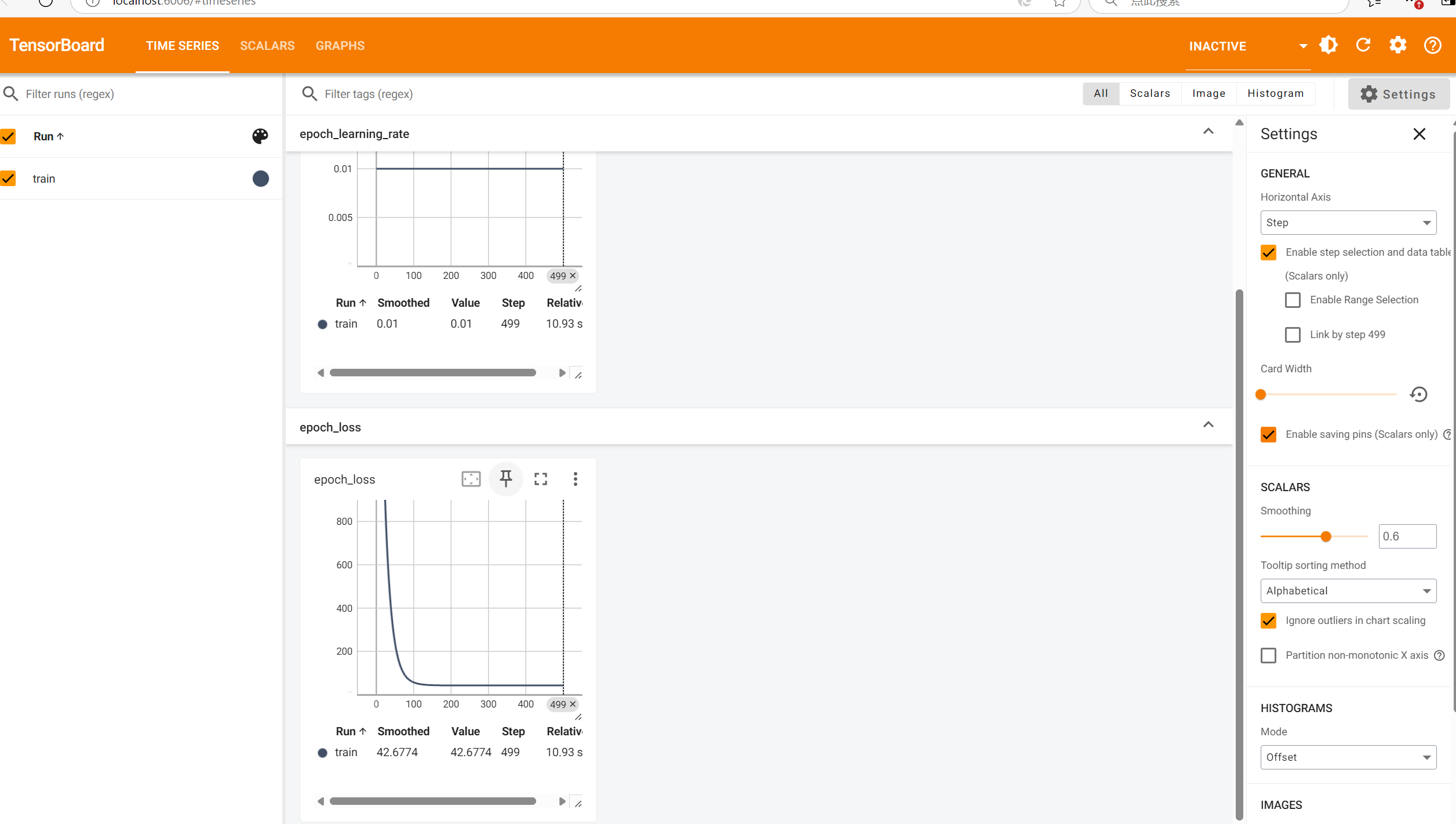
tensorboardX 可以记录和可视化模子训练过程中的指标以及模子结构。，
求换到logs路径下实行下面命令
#tensorboard --logdir ./logs
python -m tensorboard.main --logdir="./logs"
就可以通过http://localhost:6006/ 查看了

import torch # 导入torch
import numpy as np # 导入numpy
data = [[-0.5, 7.7], [1.8, 98.5], [0.9, 57.8], [0.4, 39.2], [-1.4, -15.7], [-1.4, -37.3], [-1.8, -49.1], [1.5, 75.6],
[0.4, 34.0], [0.8, 62.3]] # 定义数据集
data = np.array(data) # 将数据转换为numpy数组
x_data = data[:, 0] # 获取x坐标数据
y_data = data[:, 1] # 获取y坐标数据
x_train = torch.tensor(x_data, dtype=torch.float32) # 将x数据转换为torch张量，指定数据类型
y_train = torch.tensor(y_data, dtype=torch.float32) # 将y数据转换为torch张量，指定数据类型
print(x_train) # 打印x_train，用于调试
import torch.nn as nn # 再次导入神经网络模块，避免潜在的未定义错误
criterion = nn.MSELoss() # 定义均方误差损失函数
class LinearModel(nn.Module): # 定义线性模型
def __init__(self): # 定义初始化方法
super(
LinearModel,
self,
).__init__() # 调用父类初始化方法
self.layers = nn.Linear(1, 1) # 定义线性层，输入维度为1，输出维度为1
def forward(
self,
x
): # 定义前向传播函数
x = self.layers(x) # 将输入x通过线性层
return x # 返回输出
model = LinearModel() # 实例化线性模型
from tensorboardX import SummaryWriter # 导入SummaryWriter，用于TensorBoard可视化
writer = SummaryWriter(logdir="logs") # 创建SummaryWriter实例，指定日志存储路径
optimizer = torch.optim.SGD(model.parameters(), lr=0.01) # 定义优化器，使用随机梯度下降算法
epoches = 500 # 定义训练轮数
for n in range(1, epoches + 1): # 循环训练
y_prd = model(x_train.unsqueeze(1)) # 模型预测，unsqueeze(1)将x_train的维度从(N,)变为(N,1)
loss = criterion(y_prd.squeeze(1), y_train) # 计算损失，squeeze(1)将y_prd的维度从(N,1)变为(N,)
optimizer.zero_grad() # 梯度清零
loss.backward() # 反向传播，计算梯度
optimizer.step() # 更新模型参数
writer.add_scalar("loss", loss, n) # 将损失值写入TensorBoard
writer.add_scalar("learing_rate", optimizer.param_groups[0]["lr"], n) # 将学习率写入TensorBoard
if n % 10 == 0 or n == 1: # 每10轮打印一次损失值
print(f"epoches:{n},loss:{loss}") # 打印轮数和损失值
writer.add_graph(model, torch.rand(1, 1)) # 将模型结构写入TensorBoard
writer.close() # 关闭SummaryWriter

复制代码

四、tensorflow 框架的线性回归

从以下5个方面对深度学习框架tensorflow框架的线性回归进行介绍
1.tensorflow模子的定义
2.tensorflow模子的保存
3.tensorflow模子的加载
4.tensorflow模子网络结构的查看
5.tensorflow框架线性回归的代码实现
上面这5方面的内容，让大家，把握并理解tensorflow框架实现线性回归的过程。
tensorflow官网
https://www.tensorflow.org/guide/keras/sequential_model

https://www.tensorflow.org/guide/keras/sequential_model
下面这个网址也可以使用
Module: tf | TensorFlow v2.16.1## TensorFlow

https://tensorflow.google.cn/api_docs/python/tf

4.1 tensorflow模子的定义

什么是tf.keras？
tf.keras的功能是实现tensorflow模子搭建、模子训练和模子预测

4.1.1 tf.keras.Sequential

import tensorflow as tf
model=tf.keras.Sequential([tf.keras.layers.Dense(1,#输出特征的维度
input_shape=(1,)#输入的特征维度
)] #使用序列层需要在列表中添加线性层
)

复制代码

4.1.2 tf.keras.Sequential()另一种方式

import tensorflow as tf
#方案2的第1种方法
model=tf.keras.Sequential() #申请一个序列的对象
model.add(tf.keras.Input(shape=(1,)))
model.add(tf.keras.layers.Dense(1))
#方案2的第2种方法
model=tf.keras.Sequential()
model.add(tf.keras.layers.Dense(1,input_shape=(1,)))

复制代码

4.1.3 就是写一个类重写实现网络的搭建

import tensorflow as tf
from tensorflow.keras import Model
class Linear(Model):
#初始化
def __init__(self):
super(Linear,self).__init__()
#定义网络层
self.linear=tf.keras.layers.Dense(1)
#和pytroch有点不同，pytorch使用forward 这里使用call函数调用
def call(self,x,**kwargs):
x=self.linear(x)
return x
model=Linear()

复制代码

4.1.4 tensorflow中最常用的

import tensorflow as tf
#直接写个函数
def linear():
#input 表示输入的特征维度信息，且要指定数据类型
input=tf.keras.layers.Input(shape=(1,),dtype=tf.float32)
#下面层数搭建必须要把上一次的输入使用圆括号括起来
y=tf.keras.layers.Dense(1)(input)
#最后网络网络搭建以后必须使用tf.keras.models.Model进行封装，且输入参数(inputs)为输入的维度信息，输出参数(outputs)为最后一层网络输出
model=tf.keras.models.Model(inputs=input,outputs=y)
#返回模型
return model
model=linear()

复制代码

4.2 tensorflow模子的保存

模子的保存方式

4.2.1 保存为 .h5

HDF5文件后缀名 .h5
保存参数、模子结构、训练的设置等等
只针对函数或者顺序模子的方式 方案3不支持
model.save('./my_model.h5')

4.2.2 只保存参数

保存参数包括权重w及偏置b
model.save_weights('./model.weights.h5')

import tensorflow as tf
from tensorflow.keras import Model
#tensorflow最常用的搭建方式
#直接写个函数
def linear():
#input 表示输入的特征维度信息，且要指定数据类型
input=tf.keras.layers.Input(shape=(1,),dtype=tf.float32)
#下面层数搭建必须要把上一次的输入使用圆括号括起来
y=tf.keras.layers.Dense(1)(input)
#最后网络网络搭建以后必须使用tf.keras.models.Model进行封装，且输入参数(inputs)为输入的维度信息，输出参数(outputs)为最后一层网络输出
model=tf.keras.models.Model(inputs=input,outputs=y)
#返回模型
return model
model=linear()
model.save('./my_model.h5')
#保存为参数方式
model.save_weights('./model.weights.h5')

复制代码

4.3 tensorflow模子的加载

4.3.1 模子加载针对方式1

import tensorflow as tf
from tensorflow.keras import Model
#针对第一个方案所有的参数都保存了
# 模型的加载方式 # 方式1: HDF5文件后缀名 .h5
#加载参数、模型结构、训练的配置等等
#方式1：与pytorch区别，pytorch需要原来的模型结构，
# 在tensorflow里面可以不给原来的模型结构
load_model=tf.keras.models.load_model('my_model.h5')
print(load_model)

复制代码

4.3.2 加载只保存参数，包括权重w及偏置b

import tensorflow as tf
def linear():
#input 表示输入的特征维度信息，且要指定数据类型
input=tf.keras.layers.Input(shape=(1,),dtype=tf.float32)
#下面层数搭建必须要把上一次的输入使用圆括号括起来
y=tf.keras.layers.Dense(1)(input)
#最后网络网络搭建以后必须使用tf.keras.models.Model进行封装，且输入参数(inputs)为输入的维度信息，输出参数(outputs)为最后一层网络输出
model=tf.keras.models.Model(inputs=input,outputs=y)
#返回模型
return model
model=linear()
model.load_weights('model.weights.h5')
print(model)

复制代码

4.4 tensorflow模子网络结构的查看

4.4.1 summary() 模子搭建好就有summary()

print(model.summary())
4.4.2 使用netron

netron pycharm 终端下输入 pip install netron
下载好后，在终端下输入 netron，
在浏览器上输入 http://localhost:8080 即可
打开一个模子后刷新就可以打开另一个模子
4.4.3 最经典的 tensorboard 方法

#在计算图中添加模子
tensorboard_callback=tf.keras.callbacks.TensorBoard(log_dir='./logs')
#callbacks必要一个列表
model.fit(x_train,y_train,epochs=epochs,callbacks=[tensorboard_callback])
下载tensorboard 终端下载 pip install tensorboard ，下载成功后，切到日志写入的文件夹的上一个文件夹地点位置，输入python -m tensorboard.main --logdir="./logs" 下面会出来一个网址 http://localhost:6006/ 在浏览器打开就可以了。会显示缺少这个包，将six安装上 pip install six
结果图

模子训练好网络查看代码

#导入库
import tensorflow as tf
import numpy as np
from tensorflow.keras import Model
#设置随机化种子
seed=1
#设置随机数种子确保每次的运行结果一致
tf.random.set_seed(seed)
# 1.散点输入定义输入数据
data = [[-0.5, 7.7], [1.8, 98.5], [0.9, 57.8], [0.4, 39.2], [-1.4, -15.7], [-1.4, -37.3], [-1.8, -49.1], [1.5, 75.6], [0.4, 34.0], [0.8, 62.3]]
#转化为数组
data=np.array(data)
# 提取x 和y
x_data=data[:,0]
y_data=data[:,1]
#转化为tensorflow用的张量创建张量
x_train=tf.constant(x_data,dtype=tf.float32)
y_train=tf.constant(y_data,dtype=tf.float32)
#可以将numpy数组或者tensorflow张量把数据切成(x_train_i,y_train_i)
dataset=tf.data.Dataset.from_tensor_slices((x_train,y_train))
#shuffle是打乱，但是这个buffer_size是啥？
# buffer_size规定了乱序缓冲区的大小，且要求缓冲区大小小于或等于数据集的完整大小；
# 假设数据集的大小为10000，buffer_size为1000，最开始算法会把前1000个数据放入缓冲区；
#当从缓冲区内的这1000个数据中随机选出一个元素后，这个元素的位置会被数据集的第1001个数据替换；然后再从
#这1000个元素中随机选择第2个元素，第2个会被数据集中第1002个数据替换，以此类推，此外buffer_size不宜过大
# ，过大会导致内存爆炸
dataset=dataset.shuffle(buffer_size=10)
#数据集的batch是2
dataset=dataset.batch(2)
#预取训练的方式,CPU取数据，GPU tpu会取出来一批数据，在cpu上没效果效果会改善延迟和吞吐量
dataset=dataset.prefetch(buffer_size=tf.data.experimental.AUTOTUNE)
# 方案4
def linear():
input=tf.keras.layers.Input(shape=(1,),dtype=tf.float32)
y=tf.keras.layers.Dense(1)(input)
model=tf.keras.models.Model(inputs=input,outputs=y)
return model
model=linear()
# #3.定义损失函数和优化器
optimizer=tf.keras.optimizers.SGD(learning_rate=0.01)
#模型配置
model.compile(optimizer=optimizer,#配置优化器
loss="mean_squared_error"#配置使用什么损失函数
)
#查看网络结构
#方法1：summary()
#结构中None是batch
print(model.summary())
#方法2 使用netron
# netron pycharm 终端下输入 pip install netron
# 下载好后，在终端下输入 netron，
# 在浏览器上输入 http://localhost:8080 即可
# 打开一个模型后刷新就可以打开另一个模型
#方法 3 最经典的 tensorboard 方法
epochs=500
#在计算图中添加模型
tensorboard_callback=tf.keras.callbacks.TensorBoard(log_dir='./logs')
#callbacks需要一个列表
#模型训练
model.fit(x_train,#输入数据
y_train,#输入标签数据
epochs=epochs,#迭代的次数
callbacks=[tensorboard_callback]#图形展示可有可无
)
#保存模型
model.save_weights("model.weights.h5")
#预测模型
input_data=np.array([[-0.5]])
pre=model.predict(input_data)
#从数组中提取出结果值
print(f"model result :{pre[0][0]:2.3f}")

复制代码

总结

本文全面介绍了PyTorch和TensorFlow两大深度学习框架中模子的保存、加载以及网络结构可视化的方法。针对PyTorch，详细讲解了使用torch.save()保存和torch.load()加载整个模子以及仅保存模子参数的方法，并探究了怎样使用print(model)、torchsummary、Netron和TensorboardX等工具查看和验证模子结构。对于TensorFlow，文章阐述了使用tf.keras定义模子的三种方式，包括tf.keras.Sequential、通过类继承重写以及函数式API，并介绍了将模子保存为.h5文件和仅保存模子参数的方法。同时，本文还展示了TensorFlow模子加载以及使用summary()、Netron和TensorBoard等工具进行模子结构可视化的具体步骤。

免责声明：如果侵犯了您的权益，请联系站长，我们会及时删除侵权内容，谢谢合作！更多信息从访问主页：qidao123.com:ToB企服之家，中国第一个企服评测及商务社交产业平台。

欢迎光临 IT评测·应用市场-qidao123.com技术社区 (https://dis.qidao123.com/)