qidao123.com技术社区-IT企服评测·应用市场
标题:
第T8周:猫狗识别
[打印本页]
作者:
反转基因福娃
时间:
7 天前
标题:
第T8周:猫狗识别
● 语言环境:Python3.8.8
● 编译器:Jupyter Lab
● 深度学习环境:TensorFlow2.4.1
一、前期工作
1. 设置GPU
import tensorflow as tf
gpus = tf.config.list_physical_devices("GPU")
if gpus:
tf.config.experimental.set_memory_growth(gpus[0], True) #设置GPU显存用量按需使用
tf.config.set_visible_devices([gpus[0]],"GPU")
# 打印显卡信息,确认GPU可用
print(gpus)
复制代码
2.导入数据
import matplotlib.pyplot as plt
# 支持中文
plt.rcParams['font.sans-serif'] = ['SimHei'] # 用来正常显示中文标签
plt.rcParams['axes.unicode_minus'] = False # 用来正常显示负号
import os,PIL,pathlib
#隐藏警告
import warnings
warnings.filterwarnings('ignore')
data_dir = "./365-7-data"
data_dir = pathlib.Path(data_dir)
image_count = len(list(data_dir.glob('*/*')))
print("图片总数为:",image_count)
复制代码
二、数据预处理
1. 加载数据
使用image_dataset_from_directory方法将磁盘中的数据加载到tf.data.Dataset中
batch_size = 8
img_height = 224
img_width = 224
复制代码
"""
关于image_dataset_from_directory()的详细介绍可以参考文章:https://mtyjkh.blog.csdn.net/article/details/117018789
"""
train_ds = tf.keras.preprocessing.image_dataset_from_directory(
data_dir,
validation_split=0.2,
subset="training",
seed=12,
image_size=(img_height, img_width),
batch_size=batch_size)
复制代码
"""
关于image_dataset_from_directory()的详细介绍可以参考文章:https://mtyjkh.blog.csdn.net/article/details/117018789
"""
val_ds = tf.keras.preprocessing.image_dataset_from_directory(
data_dir,
validation_split=0.2,
subset="validation",
seed=12,
image_size=(img_height, img_width),
batch_size=batch_size)
复制代码
我们可以通过class_names输出数据集的标签。标签将按字母次序对应于目次名称。
class_names = train_ds.class_names
print(class_names)
复制代码
2.再次检查数据
for image_batch, labels_batch in train_ds:
print(image_batch.shape)
print(labels_batch.shape)
break
复制代码
● Image_batch是外形的张量(8, 224, 224, 3)。这是一批外形224x224x3的8张图片(最后一维指的是彩色通道RGB)。
● Label_batch是外形(8,)的张量,这些标签对应8张图片
3.配置数据集
● shuffle() : 打乱数据,关于此函数的具体介绍可以参考:https://zhuanlan.zhihu.com/p/42417456
● prefetch() :预取数据,加快运行,其具体介绍可以参考我前两篇文章,内里都有讲解。
● cache() :将数据集缓存到内存当中,加快运行
AUTOTUNE = tf.data.AUTOTUNE
def preprocess_image(image,label):
return (image/255.0,label)
# 归一化处理
train_ds = train_ds.map(preprocess_image, num_parallel_calls=AUTOTUNE)
val_ds = val_ds.map(preprocess_image, num_parallel_calls=AUTOTUNE)
train_ds = train_ds.cache().shuffle(1000).prefetch(buffer_size=AUTOTUNE)
val_ds = val_ds.cache().prefetch(buffer_size=AUTOTUNE)
复制代码
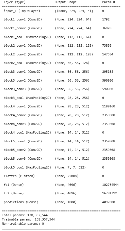
三、构建VG-16网络
from tensorflow.keras import layers, models, Input
from tensorflow.keras.models import Model
from tensorflow.keras.layers import Conv2D, MaxPooling2D, Dense, Flatten, Dropout
def VGG16(nb_classes, input_shape):
input_tensor = Input(shape=input_shape)
# 1st block
x = Conv2D(64, (3,3), activation='relu', padding='same',name='block1_conv1')(input_tensor)
x = Conv2D(64, (3,3), activation='relu', padding='same',name='block1_conv2')(x)
x = MaxPooling2D((2,2), strides=(2,2), name = 'block1_pool')(x)
# 2nd block
x = Conv2D(128, (3,3), activation='relu', padding='same',name='block2_conv1')(x)
x = Conv2D(128, (3,3), activation='relu', padding='same',name='block2_conv2')(x)
x = MaxPooling2D((2,2), strides=(2,2), name = 'block2_pool')(x)
# 3rd block
x = Conv2D(256, (3,3), activation='relu', padding='same',name='block3_conv1')(x)
x = Conv2D(256, (3,3), activation='relu', padding='same',name='block3_conv2')(x)
x = Conv2D(256, (3,3), activation='relu', padding='same',name='block3_conv3')(x)
x = MaxPooling2D((2,2), strides=(2,2), name = 'block3_pool')(x)
# 4th block
x = Conv2D(512, (3,3), activation='relu', padding='same',name='block4_conv1')(x)
x = Conv2D(512, (3,3), activation='relu', padding='same',name='block4_conv2')(x)
x = Conv2D(512, (3,3), activation='relu', padding='same',name='block4_conv3')(x)
x = MaxPooling2D((2,2), strides=(2,2), name = 'block4_pool')(x)
# 5th block
x = Conv2D(512, (3,3), activation='relu', padding='same',name='block5_conv1')(x)
x = Conv2D(512, (3,3), activation='relu', padding='same',name='block5_conv2')(x)
x = Conv2D(512, (3,3), activation='relu', padding='same',name='block5_conv3')(x)
x = MaxPooling2D((2,2), strides=(2,2), name = 'block5_pool')(x)
# full connection
x = Flatten()(x)
x = Dense(4096, activation='relu', name='fc1')(x)
x = Dense(4096, activation='relu', name='fc2')(x)
output_tensor = Dense(nb_classes, activation='softmax', name='predictions')(x)
model = Model(input_tensor, output_tensor)
return model
model=VGG16(1000, (img_width, img_height, 3))
model.summary()
复制代码
四、编译
model.compile(optimizer="adam",
loss ='sparse_categorical_crossentropy',
metrics =['accuracy'])
复制代码
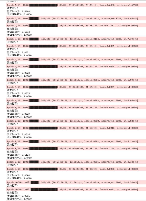
五、训练模子
from tqdm import tqdm
import tensorflow.keras.backend as K
epochs = 10
lr = 1e-4
# 记录训练数据,方便后面的分析
history_train_loss = []
history_train_accuracy = []
history_val_loss = []
history_val_accuracy = []
for epoch in range(epochs):
train_total = len(train_ds)
val_total = len(val_ds)
"""
total:预期的迭代数目
ncols:控制进度条宽度
mininterval:进度更新最小间隔,以秒为单位(默认值:0.1)
"""
with tqdm(total=train_total, desc=f'Epoch {epoch + 1}/{epochs}',mininterval=1,ncols=100) as pbar:
lr = lr*0.92
K.set_value(model.optimizer.lr, lr)
for image,label in train_ds:
"""
训练模型,简单理解train_on_batch就是:它是比model.fit()更高级的一个用法
想详细了解 train_on_batch 的同学,
可以看看我的这篇文章:https://www.yuque.com/mingtian-fkmxf/hv4lcq/ztt4gy
"""
history = model.train_on_batch(image,label)
train_loss = history[0]
train_accuracy = history[1]
pbar.set_postfix({"loss": "%.4f"%train_loss,
"accuracy":"%.4f"%train_accuracy,
"lr": K.get_value(model.optimizer.lr)})
pbar.update(1)
history_train_loss.append(train_loss)
history_train_accuracy.append(train_accuracy)
print('开始验证!')
with tqdm(total=val_total, desc=f'Epoch {epoch + 1}/{epochs}',mininterval=0.3,ncols=100) as pbar:
for image,label in val_ds:
history = model.test_on_batch(image,label)
val_loss = history[0]
val_accuracy = history[1]
pbar.set_postfix({"loss": "%.4f"%val_loss,
"accuracy":"%.4f"%val_accuracy})
pbar.update(1)
history_val_loss.append(val_loss)
history_val_accuracy.append(val_accuracy)
print('结束验证!')
print("验证loss为:%.4f"%val_loss)
print("验证准确率为:%.4f"%val_accuracy)
复制代码
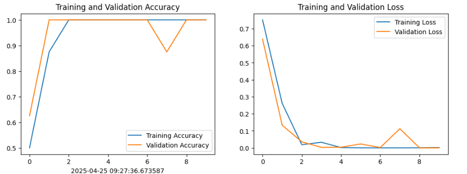
六、模子评估
from datetime import datetime
current_time = datetime.now() # 获取当前时间
epochs_range = range(epochs)
plt.figure(figsize=(12, 4))
plt.subplot(1, 2, 1)
plt.plot(epochs_range, history_train_accuracy, label='Training Accuracy')
plt.plot(epochs_range, history_val_accuracy, label='Validation Accuracy')
plt.legend(loc='lower right')
plt.title('Training and Validation Accuracy')
plt.xlabel(current_time) # 打卡请带上时间戳,否则代码截图无效
plt.subplot(1, 2, 2)
plt.plot(epochs_range, history_train_loss, label='Training Loss')
plt.plot(epochs_range, history_val_loss, label='Validation Loss')
plt.legend(loc='upper right')
plt.title('Training and Validation Loss')
plt.show()
复制代码
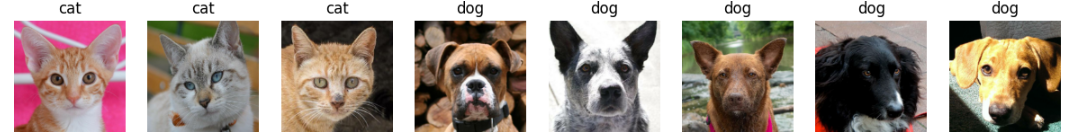
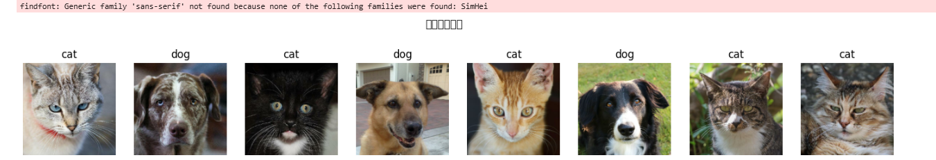
七、猜测
import numpy as np
# 采用加载的模型(new_model)来看预测结果
plt.figure(figsize=(18, 3)) # 图形的宽为18高为5
plt.suptitle("预测结果展示")
for images, labels in val_ds.take(1):
for i in range(8):
ax = plt.subplot(1,8, i + 1)
# 显示图片
plt.imshow(images[i].numpy())
# 需要给图片增加一个维度
img_array = tf.expand_dims(images[i], 0)
# 使用模型预测图片中的人物
predictions = model.predict(img_array)
plt.title(class_names[np.argmax(predictions)])
plt.axis("off")
复制代码
八、总结
VGG优缺点分析:
● VGG长处
VGG的结构非常简便,整个网络都使用了同样巨细的卷积核尺寸(3x3)和最大池化尺寸(2x2)。
● VGG缺点
1)训练时间过长,调参难度大。2)需要的存储容量大,不利于部署。比方存储VGG-16权重值文件的巨细为500多MB,不利于安装到嵌入式系统中。
结构说明:
● 13个卷积层(Convolutional Layer),分别用blockX_convX表示
● 3个全连接层(Fully connected Layer),分别用fcX与predictions表示
● 5个池化层(Pool layer),分别用blockX_pool表示
VGG的网络结构比较同一,重复使用卷积层堆叠,然后接最大池化。池化层的窗口是2x2,步长2,这样每次池化后特征图尺寸减半。然后全连接层部门有三个,最后是softmax分类。VGG16和VGG19的区别在于卷积层的数量,比如在某个块中使用2个照旧3个卷积层,大概更后面块中的数量不同。比如,VGG16的配置大概是:块1有2个卷积层,块2有2个,块3有3个,块4有3个,块5有3个,然后全连接层。而VGG19大概在这些块中多加一些卷积层,使得总层数达到19层。
免责声明:如果侵犯了您的权益,请联系站长,我们会及时删除侵权内容,谢谢合作!更多信息从访问主页:qidao123.com:ToB企服之家,中国第一个企服评测及商务社交产业平台。
欢迎光临 qidao123.com技术社区-IT企服评测·应用市场 (https://dis.qidao123.com/)
Powered by Discuz! X3.4