Python盘算机视觉编程——第二章 局部图像形貌子

1 Harris角点检测器

Harris角点检测算法是简单的角点检测算法，重要头脑是，如果像素附近表现存在多于一个方向的边，以为该点为爱好点，称为角点。
把图像域中点 x上的对称半正定矩阵                                       M                         r                              =                               M                         l                              (                      x                      )                          M_{r}=M_{l}(\mathbf{x})               Mr​=Ml​(x)界说为：
                                              M                            1                                  =                         ∇                         I                          ∇                                   I                            T                                  =                                   [                                                                                             I                                           x                                                                                                                                       I                                           y                                                                                        ]                                            [                                                                                             I                                           x                                                                                                                   I                                           y                                                                                        ]                                  =                                   [                                                                                             I                                           x                                           2                                                                                                                                   I                                              x                                                                          I                                              y                                                                                                                                                                      I                                              x                                                                          I                                              y                                                                                                                                  I                                           y                                           2                                                                                        ]                                       \boldsymbol{M}_1=\nabla\boldsymbol{I}\:\nabla\boldsymbol{I}^T=\begin{bmatrix}\boldsymbol{I}_x\\\boldsymbol{I}_y\end{bmatrix}\begin{bmatrix}\boldsymbol{I}_x&\boldsymbol{I}_y\end{bmatrix}=\begin{bmatrix}\boldsymbol{I}_x^2&\boldsymbol{I}_x\boldsymbol{I}_y\\\boldsymbol{I}_x\boldsymbol{I}_y&\boldsymbol{I}_y^2\end{bmatrix}                  M1​=∇I∇IT=[Ix​Iy​​][Ix​​Iy​​]=[Ix2​Ix​Iy​​Ix​Iy​Iy2​​]
此中                              ∇                      I                          \nabla I               ∇I 为包罗导数                                        I                         x                                  I_x               Ix​ 和                                        I                         y                                  I_\mathrm{y}               Iy​的图像梯度 。由于该界说，                                       M                         ι                                  M_{\iota}               Mι​的秩为1，特性值为                                       λ                         1                              =                      ∣                      ∇                      I                               ∣                         2                                  \lambda_1=|\nabla I|^2               λ1​=∣∇I∣2和                                       λ                         2                              =                      0                          \lambda_2=0               λ2​=0。现在对于图像的每一个像素，我们可以盘算出该矩阵。
选择权重矩阵                              W                          W               W(通常为高斯滤波器                                       G                         σ                                  G_\sigma               Gσ​),我们可以得到卷积：
                                                         M                               ‾                                      l                                  =                         W                         ∗                                   M                            l                                       \overline{M}_l=W*M_l                  Ml​=W∗Ml​
该卷积的目标是得到                                        M                         I                                  M_I               MI​ 在附近像素上的局部匀称。盘算出的矩阵                                                 M                            ‾                                  I                                  \overline{M}_I               MI​有称为 Harris矩阵。
                                                                                                                                取决于该地域                                  ∇                                  I                                   的值,Harris 矩阵                                                             M                                        ‾                                                  i                                              的特性值有三种环境                                  :                                                                                                                                                             ∙                                   如果                                                λ                                     1                                               和                                                λ                                     2                                              都是很大的正数,则该                                   x                                   点为角点                                  ;                                                                                                                                                             ∙                                   如果                                                λ                                     1                                               很大,                                               λ                                     2                                              ≈                                  0                                  ,则该地域内存在一个边,该地域内的匀称                                                M                                     i                                              的特性值不                                                                                                                                                             会变革太大;                                                                                                                                                             ∙                                   如果                                                λ                                     1                                              ≈                                               λ                                     2                                              ≈                                  0                                  ,该地域内为空。                                                                \begin{aligned}&\text{取决于该地域}\nabla\boldsymbol{I}\text{ 的值,Harris 矩阵}\overline{\boldsymbol{M}}_i\text{的特性值有三种环境}:\\&\bullet\text{ 如果 }\lambda_1\text{ 和 }\lambda_2\text{都是很大的正数,则该 }\mathbf{x}\text{ 点为角点};\\&\bullet\text{ 如果 }\lambda_1\text{ 很大,}\lambda_2\approx0\text{,则该地域内存在一个边,该地域内的匀称 }\boldsymbol{M}_i\text{的特性值不}\\&\text{会变革太大;}\\&\bullet\text{ 如果 }\lambda_1\approx\lambda_2\approx0\text{,该地域内为空。}\end{aligned}               ​取决于该地域∇I 的值,Harris 矩阵Mi​的特性值有三种环境:∙ 如果 λ1​ 和 λ2​都是很大的正数,则该 x 点为角点;∙ 如果 λ1​ 很大,λ2​≈0,则该地域内存在一个边,该地域内的匀称 Mi​的特性值不会变革太大;∙ 如果 λ1​≈λ2​≈0,该地域内为空。​

1. from matplotlib import pyplot as plt
2. from PIL import Image
3. from numpy import *
4. from numpy import random
5. from scipy.ndimage import filters
7. def compute_harris_response(img, sigma=3):
8. imgx = zeros(img.shape)
9. filters.gaussian_filter(img, (sigma, sigma), (0, 1), imgx)
10. imgy = zeros(img.shape)
11. filters.gaussian_filter(img, (sigma, sigma), (1, 0), imgy)
12. Wxx = filters.gaussian_filter(imgx * imgx, sigma)
13. Wxy = filters.gaussian_filter(imgx * imgy, sigma)
14. Wyy = filters.gaussian_filter(imgy * imgy, sigma)
15. Wdet = Wxx * Wyy - Wxy * Wxy
16. Wtran = Wxx + Wyy
17. return Wdet / Wtran
19. def get_harris_points(harrisimg, min_dist=10, threshold=0.1):
20. corners = harrisimg.max() * threshold
21. harrisimg_t = (harrisimg > corners) * 1
22. coords = array(harrisimg_t.nonzero()).T
23. candidate_values = [harrisimg[c[0], c[1]] for c in coords]
24. index = argsort(candidate_values)
25. allow_locations = zeros(harrisimg.shape)
26. allow_locations[min_dist:-min_dist, min_dist:-min_dist] = 1
27. filtered_coords = []
28. for idx in index:
29.   if allow_locations[coords[idx][0], coords[idx][1]] == 1:
30.    filtered_coords.append(coords[idx])
31.    allow_locations[coords[idx][0] - min_dist:coords[idx][0] + min_dist,
32.    coords[idx][1] - min_dist:coords[idx][1] + min_dist] = 0
33. return filtered_coords
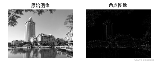
36. im = array(Image.open('jimei.jpg').convert('L'))
37. harrisim = compute_harris_response(im)
38. filtered_coords = get_harris_points(harrisim,6)
39. plt.rcParams['font.sans-serif'] = ['SimHei']
40. plt.subplot(121), plt.imshow(im, plt.cm.gray), plt.title('原始图像'), plt.axis('off')
41. plt.subplot(122), plt.imshow(harrisim, plt.cm.gray), plt.title('角点图像'), plt.axis('off')
42. plt.show()

复制代码

• 在图像间探求对应点
  Harris角点检测器仅仅可以或许检测出图像中的爱好点，没有给出通过比力图像间的爱好点来探求匹副角点的方法。须要在每个点加入形貌子信息，给出一个比力形貌子的方法。
  爱好点形貌子是分配给爱好点的一个向量，形貌该点附近的图像的表观信息。形貌子越好，探求到的对应点越好。
  

Harris 角点的形貌子通常是由附近图像像素块的灰度值，以及用于比力的归一化互
相干矩阵构成的。图像的像素块由以该像素点为中心的附近矩形部门图像构成。
通常，两个(类似巨细)像素块                                       I                         1                              (                      x                      )                          I_1(\mathbf{x})               I1​(x) 和                                       I                         2                              (                      x                      )                          I_2(\mathbf{x})               I2​(x)的相干矩阵界说为：
                                    c                         (                                   I                            1                                  ,                                   I                            2                                  )                         =                                   ∑                            x                                  f                         (                                   I                            1                                  (                         x                         )                         ,                                   I                            2                                  (                         x                         )                         )                              c(I_1,I_2)=\sum_xf(I_1(\mathbf{x}),I_2(\mathbf{x}))                  c(I1​,I2​)=x∑​f(I1​(x),I2​(x))
此中，函数                              f                          f               f随着相干方法的变革而变革。上式取像素块中全部像素位置 x的和。对于相互关矩阵，函数                              f                      (                               I                         1                              ,                               I                         2                              )                      =                               I                         1                                       I                         2                                  f(\boldsymbol I_1,\boldsymbol{I}_2)=\boldsymbol{I}_1\boldsymbol{I}_2               f(I1​,I2​)=I1​I2​,因此，                              c                      (                               I                         1                              ,                               I                         2                              )                      =                               I                         1                              ⋅                               I                         2                                  c(\boldsymbol I_1,\boldsymbol{I}_2)=\boldsymbol{I}_1\cdot\boldsymbol{I}_2               c(I1​,I2​)=I1​⋅I2​,此中·体现向量乘法(按照行大概列堆积的像素)。                              c                      (                               I                         1                              ,                               I                         2                              )                          c(I_1,I_2)               c(I1​,I2​)的值越大，像素块                                       I                         1                                  I_1               I1​和                                       I                         2                                       的相似度越高。                         1                                  I_2\text{的相似度越高。}^1               I2​的相似度越高。1
归一化的相互关矩阵是相互关矩阵的一种变形，可以界说为：
                                    n                         c                         c                                   (                                       I                               1                                      ,                                       I                               2                                      )                                  =                                   1                                       n                               −                               1                                                      ∑                            x                                                       (                                           I                                  1                                          (                               x                               )                               −                                           μ                                  1                                          )                                                 σ                               1                                            ⋅                                              (                                           I                                  2                                          (                               x                               )                               −                                           μ                                  2                                          )                                                 σ                               2                                                 ncc\left(\boldsymbol{I}_1,\boldsymbol{I}_2\right)=\frac{1}{n-1}\sum_{x}\frac{\left(\boldsymbol{I}_1(\mathbf{x})-\mu_1\right)}{\sigma_1}\cdot\frac{\left(\boldsymbol{I}_2(\mathbf{x})-\mu_2\right)}{\sigma_2}                  ncc(I1​,I2​)=n−11​x∑​σ1​(I1​(x)−μ1​)​⋅σ2​(I2​(x)−μ2​)​
此中，                              n                          n               n为像素块中像素的数量，                                       μ                         1                                  \mu_1               μ1​和                                       μ                         2                                  \mu_2               μ2​体现每个像素块中的匀称像素值强度，                                       σ                         l                                  \sigma_{\mathrm{l}}               σl​ 和                                       σ                         2                                  \sigma_{2}               σ2​分别体现每个像素块中的标准差。通过减去均值和除以标准差，该方法对图像亮度变革具有妥当性。
可以利用如下两个函数实现：

1. def get_descriptors(image, filtered_coords, wid=5):
2.     desc = []
3.     for coord in filtered_coords:
4.         patch = image[coord[0] - wid:coord[0] + wid + 1, coord[1] - wid:coord[1] + wid + 1].flatten()
5.         desc.append(patch)
6.     return desc
9. def match(desc1, desc2, threshold=0.5):
10.     n = len(desc1[0])
11.     d = -ones((len(desc1), len(desc2)))
12.     for i in range(len(desc1)):
13.         for j in range(len(desc2)):
14.             d1 = (desc1[i] - mean(desc1[i])) / std(desc1[i])
15.             d2 = (desc2[j] - mean(desc2[j])) / std(desc2[j])
16.             ncc_values = sum(d1 * d2) / (n - 1)
17.             if ncc_values > threshold:
18.                 d[i, j] = ncc_values
19.     ndx = argsort(-d)
20.     matchscores = ndx[:, 0]
21.     return matchscores

复制代码

第一个函数的参数为奇数巨细长度的方形灰度图像块，该图像块的中心为处置惩罚的像素点。该函数将图像块像素值压平成一个向量，然后添加到形貌子列表中。第二个函数利用归一化的相互关矩阵，将每个形貌子匹配到另一个图像中的最优的候选点。
2 SIFT

SIFT特性包罗爱好点检测器和形貌子。SIFT形貌子具有非常强的妥当性，SIFT特性对于标准，旋转和亮度都具有稳固性，可用于三维视角和噪声的可靠匹配。
2.1 爱好点

SIFT 特性利用高斯差分函数来定位爱好点：
                                    D                         (                         x                         ,                         σ                         )                         =                         [                                   G                                       κ                               σ                                            (                         x                         )                         −                                   G                            σ                                  (                         x                         )                         ]                         ∗                         I                         (                         x                         )                         =                         [                                   G                                       κ                               σ                                            −                                   G                            σ                                  ]                         ∗                         I                         =                                   I                                       κ                               σ                                            −                                   I                            σ                                       D(\mathbf{x},\sigma)=[G_{\kappa\sigma}(\mathbf{x})-G_{\sigma}(\mathbf{x})]*I(\mathbf{x})=[G_{\kappa\sigma}-G_{\sigma}]*I=I_{\kappa\sigma}-I_{\sigma}                  D(x,σ)=[Gκσ​(x)−Gσ​(x)]∗I(x)=[Gκσ​−Gσ​]∗I=Iκσ​−Iσ​
此中，                                       G                         σ                                  G_\sigma               Gσ​是上一章中先容的二维高斯核，                                       I                         σ                                  I_\sigma               Iσ​是利用                                       G                         σ                                  G_\sigma               Gσ​含糊的灰度图像，                              κ                          \kappa               κ是决定相差标准的常数。爱好点是在图像位置和标准变革下                              D                      (                      x                      ,                      σ                      )                          D(\mathbf{x},\sigma)               D(x,σ)的最大值和最小值点。
2.2 形貌子

为了实现旋转稳固性，基于每个点附近图像梯度的方向和巨细，SIFT形貌子引入了参考方向。SIFT形貌子利用主方向形貌参考方向。主方向利用方向直方图来度量。
2.3 检测爱好点

可以利用开源工具包VLFeat提供的二进制文件来盘算图像的SIFT特性。

1. from PIL import Image
2. from pylab import *
3. from PCV.localdescriptors import sift
4. from PCV.localdescriptors import harris
7. from matplotlib.font_manager import FontProperties
9. font = FontProperties(fname=r"c:\windows\fonts\SimSun.ttc", size=14)
11. imname = 'D:\\Python\\chapter2\\jimei2.jpg'
12. im = array(Image.open(imname).convert('L'))
13. sift.process_image(imname, 'empire.sift')
14. l1, d1 = sift.read_features_from_file('empire.sift')
16. figure()
17. gray()
18. subplot(131)
19. sift.plot_features(im, l1, circle=False)
20. title(u'(a)SIFT特征', fontproperties=font)
21. subplot(132)
22. sift.plot_features(im, l1, circle=True)
23. title(u'(b)用圆圈表示SIFT特征尺度', fontproperties=font)
25. # 检测harris角点
26. harrisim = harris.compute_harris_response(im)
28. subplot(133)
29. filtered_coords = harris.get_harris_points(harrisim, 6, 0.1)
30. imshow(im)
31. plot([p[1] for p in filtered_coords], [p[0] for p in filtered_coords], '*')
32. axis('off')
33. title(u'(c)Harris角点', fontproperties=font)
35. show()

复制代码

2.4 匹配形貌子

对于将一幅图像中的特性匹配到另一幅图像的特性，一种妥当的准则是利用这两个特性间隔和两个最匹配特性间隔的比率。

1. from PIL import Image
2. from pylab import *
3. import sys
4. from PCV.localdescriptors import sift
6. if len(sys.argv) >= 3:
7.     im1f, im2f = sys.argv[1], sys.argv[2]
8. else:
9.     im1f = 'D:\Data\xiaoqu.jpg'
10.     im2f = 'D:\Data\JiMei.jpg'
11. im1 = array(Image.open(im1f))
12. im2 = array(Image.open(im2f))
13. sift.process_image(im1f, 'out_sift_1.txt')
14. l1, d1 = sift.read_features_from_file('out_sift_1.txt')
15. figure()
16. gray()
17. subplot(121)
18. sift.plot_features(im1, l1, circle=False)
19. sift.process_image(im2f, 'out_sift_2.txt')
20. l2, d2 = sift.read_features_from_file('out_sift_2.txt')
21. subplot(122)
22. sift.plot_features(im2, l2, circle=False)
23. matches = sift.match_twosided(d1, d2)
24. print '{} matches'.format(len(matches.nonzero()[0]))
25. figure()
26. gray()
27. sift.plot_matches(im1, im2, l1, l2, matches, show_below=True)
28. show()

复制代码

免责声明：如果侵犯了您的权益，请联系站长，我们会及时删除侵权内容，谢谢合作！qidao123.com:ToB企服之家，中国第一个企服评测及软件市场,开放入驻,技术点评得现金