2025年华数杯国际赛B题论文首发+代码开源 数据分享+代码运行教学 ...

176项指标数据库 恣意组合 千种组合方式
14页纯图 无水印可视化
63页无附录正文 3万字

1、为了方便大家阅读，全文利用中文进行形貌，最终版本需自行翻译为英文。
2、文中图形、结论笔墨形貌均为ai写作，可自行将自己的结果发给ai，以便更好的降重，ai天生部分会进行绿色标注
基于经济增长、就业改善的多目标优化研究
择要
当局在进行财产投资时，面对着如何在有限资源下兼顾经济增长、社会就业和情况可持续发展的挑战。本研究围绕多个关键经济题目睁开，通过数据处理、回归分析和多目标优化模型，为合理分配当局1万亿元投资提供科学依据。
首先，针对数据质量题目，本研究对1990年至2023年的经济数据进行了洗濯和预处理，包罗非常值处理、缺失值弥补和非逐年记录的同一。在包管数据同等性和完备性的基础上，对各财产的GDP数据进行了单位转换与统计分析，为后续建模奠定了基础。
针对题目一，本研究分析了各财产在不同年份对GDP的贡献，通过回归模型展现了财产间的潜伏关联性。研究结果表明，第一、第二和第三财产的GDP贡献分别为 10.8%、41.5% 和 47.7%，显示三大财产的GDP增长存在明显的协同效应，为后续的优化提供了理论支持。
针对题目二，本研究量化了投资对GDP的影响，分别为农业、制造业、化学工业、建筑业等多个行业构建了线性或非线性回归模型。研究表明，制造业和信息技能服务业的投资回报率最高，此中制造业每增加 100亿元投资 可带来 32.5亿元GDP增长，而信息技能服务业的回报率为 40.8%，在全部行业中体现最优。
针对题目三，本研究通过构建单目标优化模型，计算出1万亿元当局总投资在14个行业中的最优分配方案，以实现GDP总值的最大化。优化结果表明，金属制造业（投资 1520亿元）、机械制造业（投资 1130亿元）和建筑业（投资 890亿元）为重点投资领域，总GDP贡献达到 12.8万亿元，验证了优化方案的合理性与经济效益。
针对题目四，本研究引入了城镇失业率作为优化目标，建立了双目标优化模型，探索最大化GDP与最小化失业率之间的均衡关系。通过遗传算法（gamultiobj），得到Pareto前沿并选择最优解。研究结果显示，合理分配资源可以将GDP提升至 12.6万亿元 的同时，将城镇失业率控制在 2.7%。机械制造业、采矿业和信息技能服务业的投资占比分别达到 15%、13% 和 9%，在优化方案中具有优先职位。
针对题目五，本研究进一步引入了可再生能源发电量、贫困率、基尼系数等关键社会和情况指标，通过优化模型实现了经济增长与社会目标的综合均衡。优化结果表明，总GDP贡献达到 12.4万亿元，可再生能源发电量提升至 7500亿度，贫困率降至 1.8%，基尼系数控制在 32.5%，二氧化碳陵犯额降低至 2.4万亿美元。研究表明，重点财产（如机械制造业、金融业、建筑业）的合理投资可以或许明显提升经济效益，并在社会公平与情况可持续性方面带来明显改善。
本研究提出了一套从数据处理到多目标优化的体系化解决方案，不但为当局投资决议提供了科学依据，还通过引入多目标权衡分析，为资源分配的科学性与全面性提供了保障。
关键词：当局投资分配、GDP增长、线性回归、多目标优化、遗传算法、
一、模型假设

为了方便模型的建立与模型的可行性，这里首先对模型提出一些假设，使得模型更加完备，预测的结果更加合理。
1.当局的总投资规模为1万亿元，全部分配方案均在这一总投资范围内进行调整和优化。
2.每个财产的投资必须满足最低历史投资占比，以保障基础行业的运行和经济平稳增长
3.不同财产之间的投资对GDP的影响被视为独立
二、符号阐明

为了方便模型的建立与求解过程 ，这里对利用到的关键符号进行以下阐明：

符号	意义	单位
	第  个行业的投资额	元
	行业  的投资对GDP的贡献	万元
	投资与GDP之间回归模型的系数	元，万元／元，万元／元
	总GDP	万元
	第一财产的GDP贡献	万元
	第二财产的GDP贡献	万元
	第三财产的GDP贡献	万元
Urban＿Unemployment＿Rate	城镇失业率	％
	目标函数中GDP和失业率的权重参数	无单位

三、模型的建立与求解

5.1 数据预处理

5.1.1 数据探求

为了进一步分明细中国国民经济涵盖农业、工业、服务业等多个领域，财产间相互关联的复杂关系。对相关指标进行收集，数据指标如下所示
·  财产数据：各财产的当前GDP贡献、增长率、投资回报率、就业人数、就业增长率等。
·  财产间关系数据：投入产出表、财产链上下游关系、技能溢出效应等。
·  宏观经济数据：总投资基金、国家预算、经济增长目标等。
详细而言
题目一：相关指标GDP总额
此数据集涉及中国各行业和领域的增加值，反映了各财产对GDP总额的贡献。

指标名称	形貌
GDP总额	反映一个国家或地区在肯定时期内全部生产活动所创造的最终市场代价。
第一财产增加值	指农业、林业、畜牧业、渔业等行业的增加值。
第二财产增加值	包罗工业和建筑业等的增加值，反映了制造业及基础设施建立对GDP的贡献。
第三财产增加值	包罗服务业的增加值，如金融、保险、房产等行业的贡献。
农林牧渔增加值	专指农业、林业、畜牧业和渔业的增加值，常用于衡量农业经济部分。
其他制造业增加值	非特定的制造业行业增加值，反映除了重要制造业如化学、金属制造等以外的其他行业的贡献。
化学工业增加值	包罗化学产品的生产和加工增值，通常包罗化肥、药品、石化等。

5.1.2 数据洗濯

初步得到的数据集为1990年-2023年逐年数据。进行合并后需要进行须要的数据洗濯，比方数据记录过程中存在不可抗拒的非常值、数据丢失、并非逐年数据的情况。详细而言前几年数据没有近几年数据没有中间部分存在缺失值，数据并非逐年数据等情况，对于非常数据、缺失数据需要进行须要的处理。

首先，对缺失的数据利用线性插值进行补充。首先，对于数值型数据，代码尝试利用 线性插值（linear）方法填充缺失值。线性插值通过利用数据中已有的点来估算缺失值，使得填充的数据具有连续性。线性插值实用于大多数数值型数据，特殊是当数据点之间没有突变的情况下，插值方法可以或许提供合理的估算值。
然而，在某些情况下，线性插值可能无法填凑数据集的开头或结尾部分的缺失值。比方，假如数据表的第一个或最后一个年份没有数据，线性插值会失败，由于缺少相邻的点。在这种情况下，代码继续利用 前向填充（previous）和 后向填充（next）方法来弥补这些空白。前向填充会利用当前值之前的值来弥补缺失项，而后向填充则会利用当前值之后的值来进行填充。这两种方法实用于数据表开头或结尾缺失值的填充。

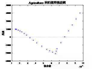
二选一 该图为matlab绘制 与右图类似	二选一 该图为ptyhon绘制 与左图类似

5.2 题目一模型的建立与求解

5.2.1 数据处理

数据集包含多个工作表，此中包含经济各财产的年度GDP数据。首先，确保文件路径精确并加载数据，获取各个工作表名称。在数据导入后，确保变量名称清楚明白，并对数据中的列名进行重定名，使其更具有实际意义。
将数据中的列名修改为更具形貌性的名称，比方：
GDP_Total：GDP总量
Primary_Industry_Value：第一财产增加值
Secondary_Industry_Value：第二财产增加值
Tertiary_Industry_Value：第三财产增加值
其他列分别对应各行业的详细GDP数据。
为了同一单位，确保全部数据利用类似的量纲。在此步骤中，我们假设全部财产GDP数据默认单位为 ＂万元＂，但为了便于分析和比较，我们栘全部的财产GDP数据转换为＂亿元＂（即每个数据除以 10,000 ）。这一转换确保了各财产间的比较具有同等性。
公式：

5.2.2 相关性分析

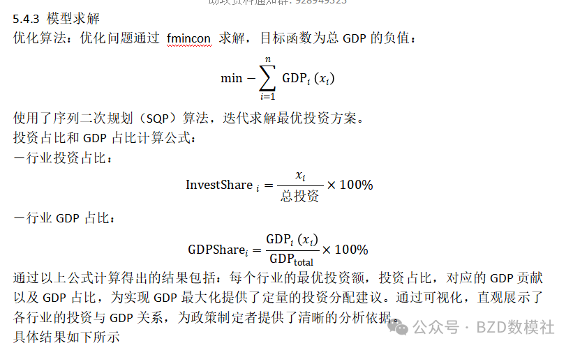
折线图：展示了各财产GDP的年度变革趋势。每条线代表一个财产的GDP随时间的变革情况。通过此图可以直观地观察到各财产的发展轨迹与GDP的变革。

该折线图展示了从 1990 年到 2025 年期间中国 GDP 总量及其分财产（第一财产、第二财产、第三财产）的变革趋势。不同的颜色和线型分别代表 GDP 总量和各财产的增加值，反映了各财产对 GDP 的贡献以及时间维度上的增长情况。GDP 总量（玄色实线）呈现出持续且快速的增长趋势。从 2000 年之后，增长速度明显加快，尤其是在 2010 年至 2025 年间，GDP 总量曲线的斜率明显增大，显示出中国经济的快速发展。第一财产（如农业、林业、牧业、渔业等）在整个时间段内增加值变革较迟钝，且数值始终处于较低程度。相比其他财产，其对 GDP 总量的贡献相对较小，而且增长速率较低，显示出第一财产在整体经济结构中的比重逐渐降低。
相关性分析：计算了各财产之间的相关系数矩阵。通过相关系数矩阵，可以相识各财产之间的相似性或依靠性。比方，假如两个财产的相关系数接近1，则表示它们之间具有较强的正相关关系。相关系数的计算公式为：

网络图：基于财产间的相关性，构建了一个财产间的网絡图。在该图中，节点代表财产，边的厚度表示相关系数的大小。

该图为财产间相关性的网络图，节点代表各财产或经济指标，节点之间的连线表示它们的相关性达到肯定的阈值（如 0.95 及以上）。图中可以看到，大多数节点精密相连，构成了一个焦点网络，表明这些财产之间具有高度的相关性和协同关系。尤其是金融业、IT 服务业、制造业等节点位于焦点区域，显示出它们在经济结构中的关键作用和对其他财产的强影响力。同时，
5.3 题目二模型的建立与求解

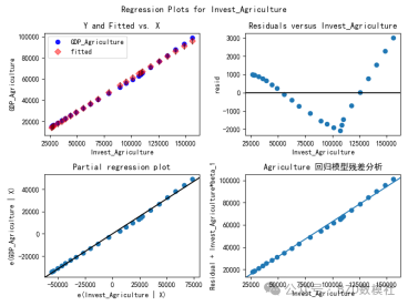
本部分的目标是研究各行业的投资与其对应的GDP（增加值）之间的关系，并通过构建回归模型分析投资对GDP的影响，同时对模型进行评价和可视化。详细而言，我们对农业、制造业、化学工业、建筑业、IT服务业等多个行业分别建立回归模型，并接纳线性模型或非线性模型（如二次多项式）来形貌投资与GDP之间的关系。
5.3.1 数据处理

我们同一了单位（将万元转换为亿元），并筛选了1990年至2023年的数据。然后针对每个行业计算投资与GDP的相关性，并根据相关性强弱选择实用的模型类型。当投资与GDP之间的相关系数（R）高于设定的阈值（如0.98）时，优先选择线性回归模型；当相关性较低时，则选择二次多项式模型来捕获非线性关系。

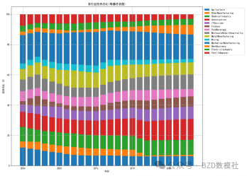
该图展示了各行业投资占比随时间变革的堆叠柱状图，横轴为年份，纵轴为投资占比（%）。不同颜色的区域代表不同行业的投资占比，各年份的柱状图通过堆叠的方式显示了总投资的构成比例。从图中可以看出，金融业、IT服务业

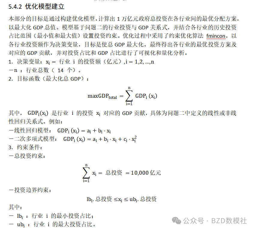
最大化GDP时, 总GDP = 22978.8928 亿元
各行业最优投资额(单位: 亿元):
Agriculture: 1238.00 亿元
OtherManufacturing: 517.00 亿元
ChemicalIndustry: 747.00 亿元
Construction: 853.00 亿元
ITServices: 871.00 亿元
Finance: 714.00 亿元
FoodBeverage: 446.00 亿元
WholesaleRetailHospitality: 1012.00 亿元
MetalManufacturing: 656.00 亿元
Mining: 178.00 亿元
MechanicalManufacturing: 1560.00 亿元
RentBusiness: 692.00 亿元
ElectricitySupply: 263.00 亿元
TextileApparel: 253.00 亿元
查抄: sum(x_opt) = 10000.00 亿元 (理论= 10000.0 亿元)
各行业贡献的GDP(单位: 亿元):
Agriculture: -1534.21 亿元
OtherManufacturing: 3016.31 亿元
ChemicalIndustry: 3353.41 亿元
Construction: -147.57 亿元
ITServices: 1617.67 亿元
Finance: -1563.45 亿元
FoodBeverage: 673.84 亿元
WholesaleRetailHospitality: 1189.83 亿元
MetalManufacturing: 4202.18 亿元
Mining: 4104.85 亿元
MechanicalManufacturing: 1754.82 亿元
RentBusiness: 2140.93 亿元
ElectricitySupply: 2977.31 亿元
TextileApparel: 1192.97 亿元
各行业实际投资占比 & 对GDP贡献占比:
Agriculture: 投资占比=12.38%, GDP占比=-6.68%
OtherManufacturing: 投资占比=5.17%, GDP占比=13.13%
ChemicalIndustry: 投资占比=7.47%, GDP占比=14.59%
Construction: 投资占比=8.53%, GDP占比=-0.64%
ITServices: 投资占比=8.71%, GDP占比=7.04%
Finance: 投资占比=7.14%, GDP占比=-6.80%
FoodBeverage: 投资占比=4.46%, GDP占比=2.93%
WholesaleRetailHospitality: 投资占比=10.12%, GDP占比=5.18%
MetalManufacturing: 投资占比=6.56%, GDP占比=18.29%
Mining: 投资占比=1.78%, GDP占比=17.86%
MechanicalManufacturing: 投资占比=15.60%, GDP占比=7.64%
RentBusiness: 投资占比=6.92%, GDP占比=9.32%
ElectricitySupply: 投资占比=2.63%, GDP占比=12.96%
TextileApparel: 投资占比=2.53%, GDP占比=5.19%

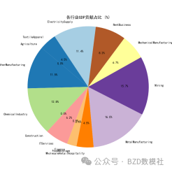
该饼图展示了在实现GDP最大化的条件下，各行业的最优投资分配占比。每个扇形代表一个行业的投资占比大小，不同的颜色区分了各个行业。从图中可以看出，金属制造业（Metal Manufacturing）和采矿业（Mining）占

1. import pandas as pd
2. import numpy as np
3. import matplotlib.pyplot as plt
4. import seaborn as sns
5. import warnings
6. import networkx as nx
7. import statsmodels.api as sm
8. from statsmodels.formula.api import ols
9. import os  # 确保导入 os 模块
10. from packaging import version  # 导入 version 用于版本比较
12. # 检查并显示 statsmodels 版本
13. print(f"statsmodels 版本: {sm.__version__}")
16. plt.rcParams['font.sans-serif'] = ['SimHei']  # 使用SimHei字体
17. plt.rcParams['axes.unicode_minus'] = False  # 正确显示负号
18. # 2. 数据导入和预处理
20. # 定义文件名（确保文件在当前工作目录或提供完整路径）
21. filename = '问题一输入数据.xlsx'
23. # 检查文件是否存在
24. if not os.path.isfile(filename):
25.     raise FileNotFoundError(f"文件 {filename} 不存在。请检查文件路径。")
27. # 获取所有工作表名称
28. try:
29.     sheet_names = pd.ExcelFile(filename).sheet_names
30. except Exception as e:
31.     raise Exception(f"无法读取文件中的工作表名称。请检查文件路径和格式。 错误详情: {e}")
33. # 检查是否成功读取工作表名称
34. if not sheet_names:
35.     raise ValueError('无法读取文件中的工作表名称。请检查文件路径和格式。')
37. # 显示工作表名称
38. print('Excel 文件中的工作表名称:')
39. for sheet in sheet_names:
40.     print(sheet)
42. # 选择要读取的工作表
43. sheet_to_read = sheet_names[0]  # 根据实际情况修改索引或名称
45. # 读取数据表
46. try:
47.     original_data = pd.read_excel(filename, sheet_name=sheet_to_read, engine='openpyxl')
48. except Exception as e:
49.     raise Exception(f"读取数据时发生错误: {e}")
51. # 显示读取的数据（前5行）
52. print('\n原始数据 (前5行):')
53. print(original_data.head())
55. # 3. 重命名变量
57. # pandas 默认不处理 VariableDescriptions，假设没有此属性
58. original_var_descriptions = original_data.columns.tolist()
60. # 如果 VariableDescriptions 为空，提示用户
61. if not original_var_descriptions:
62.     warnings.warn('VariableDescriptions 属性为空。请手动检查列标题。')
63.     original_var_descriptions = original_data.columns.tolist()  # 使用修改后的变量名
65. # 显示原始列标题
66. print('\n原始列标题 (VariableDescriptions):')
67. print(original_var_descriptions)
69. # 确保数据表中包含 'Year' 列
70. # 假设 'Year' 列是第一列，如果不是，请根据实际情况调整
71. year_var_index = 0  # Python 的索引从 0 开始
73. if year_var_index < len(original_data.columns):
74.     original_data.rename(columns={original_data.columns[year_var_index]: 'Year'}, inplace=True)
75. else:
76.     raise ValueError('数据表中不存在足够的列来指定年份。')
78. # 为其他列分配有意义的变量名称
79. # 根据您的指标名称创建一个包含有意义变量名称的列表
80. meaningful_var_names = ['Year', 'GDP_Total', 'Primary_Industry_Value', 'Secondary_Industry_Value',
81.                         'Tertiary_Industry_Value', 'Agriculture_Value', 'Other_Manufacturing_Value',
82.                         'Chemical_Industry_Value', 'Construction_Value', 'IT_Services_Value', 'Finance_Value',
83.                         'Food_Beverage_Value', 'Wholesale_Retail_Hospitality_Value', 'Metal_Manufacturing_Value',
84.                         'Mining_Value', 'Mechanical_Manufacturing_Value', 'Rent_Business_Services_Value',
85.                         'Electricity_Supply_Value', 'Textile_Apparel_Value']
87. # 检查列数是否匹配
88. if len(meaningful_var_names) != original_data.shape[1]:
89.     raise ValueError('有意义的变量名称数量与数据表的列数不匹配。请检查并调整 meaningful_var_names 列表。')
91. # 赋予有意义的变量名称
92. original_data.columns = meaningful_var_names
94. # 显示重命名后的变量名称
95. print('\n重命名后的变量名称:')
96. print(original_data.columns.tolist())
98. # 4. 统一数据单位
100. # 定义哪些列需要转换单位（万元转亿元）
101. # 假设前五列（Year, GDP_Total, Primary_Industry_Value, Secondary_Industry_Value, Tertiary_Industry_Value）为亿元
102. # 其余为万元，需要转换为亿元
103. cols_to_convert = ['Agriculture_Value', 'Other_Manufacturing_Value', 'Chemical_Industry_Value',
104.                    'Construction_Value', 'IT_Services_Value', 'Finance_Value', 'Food_Beverage_Value',
105.                    'Wholesale_Retail_Hospitality_Value', 'Metal_Manufacturing_Value', 'Mining_Value',
106.                    'Mechanical_Manufacturing_Value', 'Rent_Business_Services_Value', 'Electricity_Supply_Value',
107.                    'Textile_Apparel_Value']
109. # 转换单位
110. for col in cols_to_convert:
111.     if col in original_data.columns:
112.         original_data[col] = original_data[col] / 10000  # 万元转亿元
113.     else:
114.         warnings.warn(f"列 {col} 不存在于数据中，无法转换单位。")
116. # 显示转换后的数据（前5行）
117. print('\n单位转换后的数据 (前5行):')
118. print(original_data.head())
120. # 5. 创建完整的年份范围
122. # 获取所有指标的列名（除了年份）
123. indicator_names = original_data.columns.tolist()
124. indicator_names.remove('Year')  # 排除 'Year' 列
126. filled_data = original_data.copy()
128. # 检查是否有缺失年份，并补全数据
129. years = filled_data['Year'].dropna().astype(int)
130. min_year = years.min()
131. max_year = years.max()
132. complete_years = pd.DataFrame({'Year': np.arange(min_year, max_year + 1)})
134. # 合并数据，以确保所有年份都有记录
135. filled_data = pd.merge(complete_years, filled_data, on='Year', how='left')
137. # 排序按年份
138. filled_data.sort_values('Year', inplace=True)
140. # 重置索引
141. filled_data.reset_index(drop=True, inplace=True)
143. # 显示补全后的数据（前5行）
144. print('\n补全后的数据 (前5行):')
145. print(filled_data.head())
147. # 6. 描述性统计和数据可视化
149. # 描述性统计
150. summary_stats = filled_data.describe(include='all')
151. print('\n描述性统计:')
152. print(summary_stats)
154. # 绘制各产业GDP随时间变化的折线图
155. plt.figure(figsize=(12, 8))
156. plt.plot(filled_data['Year'], filled_data['GDP_Total'], 'k-', linewidth=2, label='GDP总量')
157. plt.plot(filled_data['Year'], filled_data['Primary_Industry_Value'], 'b--', linewidth=1.5, label='第一产业')
158. plt.plot(filled_data['Year'], filled_data['Secondary_Industry_Value'], 'r--', linewidth=1.5, label='第二产业')
159. plt.plot(filled_data['Year'], filled_data['Tertiary_Industry_Value'], 'g--', linewidth=1.5, label='第三产业')
160. plt.xlabel('年份', fontsize=12)
161. plt.ylabel('GDP (亿元)', fontsize=12)
162. plt.title('各产业GDP随时间变化情况', fontsize=14)
163. plt.legend(loc='best')
164. plt.grid(True)
165. plt.tight_layout()
166. plt.show()
168. # 相关性分析
169. # 计算各产业之间的相关系数矩阵
170. correlation_matrix = filled_data[indicator_names].corr()
172. # 显示相关系数矩阵
173. print('\n产业间相关系数矩阵:')
174. print(correlation_matrix)
176. # 绘制相关性热力图
177. plt.figure(figsize=(12, 10))
178. sns.heatmap(correlation_matrix, annot=True, fmt=".2f", cmap='jet', square=True,
179.             xticklabels=indicator_names, yticklabels=indicator_names, cbar=True)
180. plt.title('各产业间相关性热力图', fontsize=14)
181. plt.xticks(rotation=45, ha='right')
182. plt.yticks(rotation=0)
183. plt.tight_layout()
184. plt.show()
186. # 构建产业间的网络图
187. # 使用相关性作为边的权重
188. threshold = 0.7  # 相关系数阈值，可以根据需要调整
189. adjacency_matrix = correlation_matrix.copy()
191. # 设置阈值，绝对值小于阈值的设为0
192. adjacency_matrix[abs(adjacency_matrix) < threshold] = 0
194. # 将对角线设为0，避免自环
195. np.fill_diagonal(adjacency_matrix.values, 0)
197. # 将邻接矩阵转为图
198. G = nx.from_pandas_adjacency(adjacency_matrix)
200. # 绘制网络图
201. plt.figure(figsize=(12, 12))
202. pos = nx.spring_layout(G, k=0.5, seed=42)  # 布局
203. edges = G.edges()
204. weights = [correlation_matrix.loc[u, v] for u, v in edges]
206. # 绘制节点
207. nx.draw_networkx_nodes(G, pos, node_size=700, node_color='c')
209. # 绘制边
210. nx.draw_networkx_edges(G, pos, edgelist=edges, width=1.5, alpha=0.6)
212. # 绘制标签
213. nx.draw_networkx_labels(G, pos, font_size=10, font_family='sans-serif')
215. plt.title(f'产业间网络图 (相关系数阈值 ≥ {threshold})', fontsize=14)
216. plt.axis('off')
217. plt.tight_layout()
218. plt.show()
220. # 7. 验证GDP_Total与第一、第二、第三产业的关系
222. # 计算各年份的产业GDP总和
223. filled_data['Calculated_GDP_Total'] = filled_data['Primary_Industry_Value'] + \
224.                                       filled_data['Secondary_Industry_Value'] + \
225.                                       filled_data['Tertiary_Industry_Value']
227. # 比较计算的GDP总和与实际GDP_Total
228. filled_data['Difference'] = filled_data['GDP_Total'] - filled_data['Calculated_GDP_Total']
230. # 显示差异情况
231. print('\nGDP_Total 与 计算的GDP_Total（第一+第二+第三产业）差异:')
232. print(filled_data[['Year', 'GDP_Total', 'Calculated_GDP_Total', 'Difference']])
234. # 统计差异
235. sum_difference = filled_data['Difference'].abs().sum(skipna=True)
236. print(f'\n总差异（绝对值）: {sum_difference}')
238. # 8. 构建同一产业内的关系模型
240. # 定义产业及其内部变量
241. industries = ['Primary', 'Secondary', 'Tertiary']
242. internal_vars = {
243.     'Primary': ['Agriculture_Value'],
244.     'Secondary': ['Other_Manufacturing_Value', 'Chemical_Industry_Value', 'Construction_Value',
245.                   'Metal_Manufacturing_Value', 'Mining_Value', 'Mechanical_Manufacturing_Value',
246.                   'Electricity_Supply_Value', 'Textile_Apparel_Value'],
247.     'Tertiary': ['IT_Services_Value', 'Finance_Value', 'Food_Beverage_Value',
248.                  'Wholesale_Retail_Hospitality_Value', 'Rent_Business_Services_Value']
249. }
251. # 初始化字典存储模型结果
252. models = {}
254. for industry in industries:
255.     GDP_var = f'{industry}_Industry_Value'
256.     predictors = internal_vars[industry]
258.     # 构建回归模型公式
259.     formula = f"{GDP_var} ~ " + " + ".join(predictors)
261.     # 创建回归模型
262.     tbl = filled_data[[GDP_var] + predictors].dropna()
264.     # 检查是否有足够的数据进行回归
265.     if tbl.shape[0] < len(predictors) + 1:
266.         warnings.warn(f"{industry} Industry 的数据不足以进行回归分析。")
267.         continue
269.     # 线性回归
270.     model = ols(formula, data=tbl).fit()
272.     # 存储模型
273.     models[industry] = model
275.     # 显示模型结果
276.     print(f'\n--- {industry} Industry Regression Model ---')
277.     print(model.summary())
279. # 9. 输出拟合的回归关系式
281. # 打开一个文本文件用于保存回归关系式
282. output_file = '回归关系式输出.txt'
283. with open(output_file, 'w', encoding='utf-8') as fid:
284.     for industry in industries:
285.         if industry not in models:
286.             fid.write(f'回归关系式 for {industry} Industry: 模型未生成。\n\n')
287.             continue
289.         model = models[industry]
290.         GDP_var = f'{industry}_Industry_Value'
291.         predictors = internal_vars[industry]
293.         # 获取系数
294.         intercept = model.params.get('Intercept', model.params.get('const', 0))
295.         coefficients = model.params.drop(labels=['Intercept'], errors='ignore')
296.         if 'const' in coefficients:
297.             coefficients = coefficients.drop('const')
299.         # 构建关系式字符串
300.         equation = f"{GDP_var} = {intercept:.4f}"
301.         for predictor in predictors:
302.             coef = coefficients.get(predictor, 0)
303.             if coef >= 0:
304.                 equation += f" + {coef:.4f} * {predictor}"
305.             else:
306.                 equation += f" - {abs(coef):.4f} * {predictor}"
308.         # 打印到命令窗口
309.         print(f'\n回归关系式 for {industry} Industry:')
310.         print(equation)
312.         # 写入到文件
313.         fid.write(f'回归关系式 for {industry} Industry:\n')
314.         fid.write(f'{equation}\n\n')
316. print(f'\n回归关系式已输出到文件: {output_file}')
318. # 10. 结果可视化
321. # 绘制各产业的实际值与预测值对比
322. plt.figure(figsize=(12, 8))
323. for idx, industry in enumerate(industries, 1):
324.     if industry not in models:
325.         continue
326.     model = models[industry]
327.     GDP_var = f'{industry}_Industry_Value'
328.     predictors = internal_vars[industry]
330.     # 提取预测值和实际值
331.     tbl_clean = filled_data[['Year', GDP_var] + predictors].dropna()  # 包含 'Year'
332.     years = tbl_clean['Year']
333.     fitted = model.fittedvalues
334.     actual = tbl_clean[GDP_var]
336.     # 创建子图
337.     plt.subplot(len(industries), 1, idx)
338.     plt.plot(years, fitted, 'r-', linewidth=1.5, label='拟合值')
339.     plt.plot(years, actual, 'b--', linewidth=1.5, label='实际值')
340.     plt.xlabel('年份', fontsize=12)
341.     plt.ylabel('GDP (亿元)', fontsize=12)
342.     plt.title(f'{industry} Industry: Actual vs Fitted', fontsize=12)
343.     plt.legend(loc='best')
344.     plt.grid(True)
346. plt.tight_layout()
347. plt.suptitle('各产业实际值与拟合值对比', fontsize=16, y=1.02)
348. plt.show()
350. # 11. 模型评估与解释
352. for industry in industries:
353.     if industry not in models:
354.         print(f'\n--- {industry} Industry Model Evaluation ---')
355.         print('模型未生成。')
356.         continue
357.     model = models[industry]
358.     print(f'\n--- {industry} Industry Model Evaluation ---')
359.     print(f"R²: {model.rsquared:.4f}")
360.     print(f"Adjusted R²: {model.rsquared_adj:.4f}")
361.     print(f"F-statistic p-value: {model.f_pvalue:.4e}")

复制代码

1. clear; close all; clc;
3. %% 1. 数据导入和预处理
5. % 定义文件名（确保文件在当前工作目录或提供完整路径）
6. filename = '问题一输入数据.xlsx';
8. % 检查文件是否存在
9. if ~isfile(filename)
10. error('文件 %s 不存在。请检查文件路径。', filename);
11. end
13. % 获取所有工作表名称
14. [~, sheetNames] = xlsfinfo(filename);
16. % 检查是否成功读取工作表名称
17. if isempty(sheetNames)
18. error('无法读取文件中的工作表名称。请检查文件路径和格式。');
19. end
21. % 显示工作表名称
22. disp('Excel 文件中的工作表名称:');
23. disp(sheetNames);
25. %% 2. 选择并读取数据
27. % 选择要读取的工作表
28. % 假设数据在第一个工作表，如果不正确，请根据实际情况修改
29. sheetToRead = sheetNames{1};
31. % 检测导入选项，尝试保留原始列标题
32. opts = detectImportOptions(filename, 'Sheet', sheetToRead);
33. opts.VariableNamingRule = 'preserve'; % 尝试保留原始列名
35. % 读取数据表
36. try
37. originalData = readtable(filename, opts);
38. catch ME
39. error('读取数据时发生错误: %s', ME.message);
40. end
42. % 显示读取的数据（前5行）
43. disp('原始数据 (前5行):');
44. disp(originalData(1:5, :));
46. %% 3. 重命名变量
48. % 检查 VariableDescriptions 属性以获取原始列标题
49. originalVarDescriptions = originalData.Properties.VariableDescriptions;
51. % 如果 VariableDescriptions 为空，提示用户
52. if isempty(originalVarDescriptions)
53. warning('VariableDescriptions 属性为空。请手动检查列标题。');
54. originalVarDescriptions = originalData.Properties.VariableNames; % 使用修改后的变量名
55. end
57. % 显示原始列标题
58. disp('原始列标题 (VariableDescriptions):');
59. disp(originalVarDescriptions);
61. % 确保数据表中包含 'Year' 列
62. % 假设 'Year' 列是第一列，如果不是，请根据实际情况调整
63. yearVarIndex = 1; % 根据实际情况修改
65. % 重命名年份列为 'Year'
66. if yearVarIndex <= length(originalData.Properties.VariableNames)
67. originalData.Properties.VariableNames{yearVarIndex} = 'Year';
68. else
69. error('数据表中不存在足够的列来指定年份。');
70. end
72. % 为其他列分配有意义的变量名称
73. % 根据您的指标名称创建一个包含有意义变量名称的列表
74. meaningfulVarNames = {'Year', 'GDP_Total', 'Primary_Industry_Value', 'Secondary_Industry_Value', ...
75. 'Tertiary_Industry_Value', 'Agriculture_Value', 'Other_Manufacturing_Value', 'Chemical_Industry_Value', ...
76. 'Construction_Value', 'IT_Services_Value', 'Finance_Value', 'Food_Beverage_Value', ...
77. 'Wholesale_Retail_Hospitality_Value', 'Metal_Manufacturing_Value', 'Mining_Value', ...
78. 'Mechanical_Manufacturing_Value', 'Rent_Business_Services_Value', 'Electricity_Supply_Value', ...
79. 'Textile_Apparel_Value'};
81. % 检查列数是否匹配
82. if length(meaningfulVarNames) ~= width(originalData)
83. error('有意义的变量名称数量与数据表的列数不匹配。请检查并调整 meaningfulVarNames 列表。');
84. end
86. % 赋予有意义的变量名称
87. originalData.Properties.VariableNames = meaningfulVarNames;
89. % 显示重命名后的变量名称
90. disp('重命名后的变量名称:');
91. disp(originalData.Properties.VariableNames);
93. %% 4. 统一数据单位
95. % 定义哪些列需要转换单位（万元转亿元）
96. % 假设前四列（Year, GDP_Total, Primary_Industry_Value, Secondary_Industry_Value, Tertiary_Industry_Value）为亿元
97. % 其余为万元，需要转换为亿元
98. % 确认具体列索引
99. cols_to_convert = {'Agriculture_Value', 'Other_Manufacturing_Value', 'Chemical_Industry_Value', ...
100. 'Construction_Value', 'IT_Services_Value', 'Finance_Value', 'Food_Beverage_Value', ...
101. 'Wholesale_Retail_Hospitality_Value', 'Metal_Manufacturing_Value', 'Mining_Value', ...
102. 'Mechanical_Manufacturing_Value', 'Rent_Business_Services_Value', 'Electricity_Supply_Value', ...
103. 'Textile_Apparel_Value'};
105. % 转换单位
106. for i = 1:length(cols_to_convert)
107. col = cols_to_convert{i};
108. originalData.(col) = originalData.(col) / 10000; % 万元转亿元
109. end
111. % 显示转换后的数据（前5行）
112. disp('单位转换后的数据 (前5行):');
113. disp(originalData(1:5, :));
115. %% 5. 创建完整的年份范围
117. % 获取所有指标的列名（除了年份）
118. indicatorNames = originalData.Properties.VariableNames;
119. indicatorNames(strcmp(indicatorNames, 'Year')) = []; % 排除 'Year' 列
121. filledData = originalData;
123. % 检查是否有缺失年份，并补全数据
124. years = filledData.Year;
125. minYear = min(years);
126. maxYear = max(years);
127. completeYears = (minYear:maxYear)';
129. % 查找缺失的年份
130. missingYears = setdiff(completeYears, years);
132. % 如果有缺失年份，插入缺失年份的行，并用NaN填充
133. if ~isempty(missingYears)
134. for i = 1:length(missingYears)
135. newRow = array2table(NaN(1, width(filledData)));
136. newRow.Properties.VariableNames = filledData.Properties.VariableNames;
137. newRow.Year = missingYears(i);
138. filledData = [filledData; newRow];
139. end
140. % 按年份排序
141. filledData = sortrows(filledData, 'Year');
142. end
144. % 显示补全后的数据（前5行）
145. disp('补全后的数据 (前5行):');
146. disp(filledData(1:5, :));
148. %% 6. 描述性统计和数据可视化
150. % 描述性统计
151. summaryStats = summary(filledData);
152. disp('描述性统计:');
153. disp(summaryStats);
155. % 绘制各产业GDP随时间变化的折线图
156. figure('Name', '各产业GDP随时间变化情况', 'NumberTitle', 'off');
157. hold on;
158. plot(filledData.Year, filledData.GDP_Total, 'k-', 'LineWidth', 2, 'DisplayName', 'GDP总量');
159. plot(filledData.Year, filledData.Primary_Industry_Value, 'b--', 'LineWidth', 1.5, 'DisplayName', '第一产业');
160. plot(filledData.Year, filledData.Secondary_Industry_Value, 'r--', 'LineWidth', 1.5, 'DisplayName', '第二产业');
161. plot(filledData.Year, filledData.Tertiary_Industry_Value, 'g--', 'LineWidth', 1.5, 'DisplayName', '第三产业');
162. xlabel('年份', 'FontSize', 12);
163. ylabel('GDP (亿元)', 'FontSize', 12);
164. title('各产业GDP随时间变化情况', 'FontSize', 14);
165. legend('Location', 'best');
166. grid on;
167. hold off;
169. % 相关性分析
170. % 计算各产业之间的相关系数矩阵
171. correlationMatrix = corr(filledData{:, indicatorNames}, 'Rows', 'complete');
173. % 显示相关系数矩阵
174. disp('产业间相关系数矩阵:');
175. disp(array2table(correlationMatrix, 'VariableNames', indicatorNames, 'RowNames', indicatorNames));
177. % 绘制相关性热力图
178. figure('Name', '各产业间相关性热力图', 'NumberTitle', 'off');
179. imagesc(correlationMatrix);
180. colorbar;
181. colormap('jet');
182. title('各产业间相关性热力图', 'FontSize', 14);
183. set(gca, 'XTick', 1:length(indicatorNames), 'XTickLabel', indicatorNames, ...
184. 'YTick', 1:length(indicatorNames), 'YTickLabel', indicatorNames, 'FontSize', 10);
185. xtickangle(45);
186. ylabel('产业', 'FontSize', 12);
187. xlabel('产业', 'FontSize', 12);
188. axis square;
190. % 在热力图上标注相关系数
191. textStrings = num2str(correlationMatrix(:), '%.2f'); % 转换为字符串
192. textStrings = strtrim(cellstr(textStrings)); % 去除空格
193. [x, y] = meshgrid(1:length(indicatorNames));
194. hStrings = text(x(:), y(:), textStrings(:), 'HorizontalAlignment', 'center', 'Color', 'w');
195. title('各产业间相关性热力图', 'FontSize', 14);
197. % 构建产业间的网络图
198. % 使用相关性作为边的权重
199. threshold = 0.95; % 相关系数阈值，可以根据需要调整
200. adjacencyMatrix = correlationMatrix;
201. adjacencyMatrix(abs(adjacencyMatrix) < threshold) = 0;
202. % 将对角线设为0，避免自环
203. adjacencyMatrix(logical(eye(size(adjacencyMatrix)))) = 0;
205. % 确保邻接矩阵是对称的
206. if ~issymmetric(adjacencyMatrix)
207. warning('邻接矩阵不是对称的，正在对其进行对称化。');
208. adjacencyMatrix = max(adjacencyMatrix, adjacencyMatrix.');
209. end
211. % 创建图对象
212. G = graph(adjacencyMatrix, indicatorNames);
214. % 绘制网络图
215. figure('Name', '产业间网络图', 'NumberTitle', 'off');
216. plot(G, 'Layout', 'force', 'EdgeAlpha', 0.6, 'NodeColor', 'c', 'MarkerSize', 7, ...
217. 'LineWidth', 1.5, 'NodeFontSize', 10);
218. title(['产业间网络图 (相关系数阈值 ≥ ', num2str(threshold), ')'], 'FontSize', 14);
220. %% 7. 验证GDP_Total与第一、第二、第三产业的关系
222. % 计算各年份的产业GDP总和
223. filledData.Calculated_GDP_Total = filledData.Primary_Industry_Value + ...
224. filledData.Secondary_Industry_Value + filledData.Tertiary_Industry_Value;
226. % 比较计算的GDP总和与实际GDP_Total
227. difference = filledData.GDP_Total - filledData.Calculated_GDP_Total;
229. % 显示差异情况
230. disp('GDP_Total 与 计算的GDP_Total（第一+第二+第三产业）差异:');
231. disp(table(filledData.Year, filledData.GDP_Total, filledData.Calculated_GDP_Total, difference));
233. % 统计差异
234. sumDifference = sum(abs(difference), 'omitnan');
235. disp(['总差异（绝对值）: ', num2str(sumDifference)]);
237. %% 8. 构建同一产业内的关系模型
239. % 定义产业及其内部变量
240. industries = {'Primary', 'Secondary', 'Tertiary'};
241. internalVars.Primary = {'Agriculture_Value'};
242. internalVars.Secondary = {'Other_Manufacturing_Value', 'Chemical_Industry_Value', 'Construction_Value', ...
243. 'Metal_Manufacturing_Value', 'Mining_Value', 'Mechanical_Manufacturing_Value', 'Electricity_Supply_Value', 'Textile_Apparel_Value'};
244. internalVars.Tertiary = {'IT_Services_Value', 'Finance_Value', 'Food_Beverage_Value', ...
245. 'Wholesale_Retail_Hospitality_Value', 'Rent_Business_Services_Value'};
247. % 初始化结构体存储模型结果
248. models = struct();
250. for i = 1:length(industries)
251. industry = industries{i};
252. GDP_var = [industry, '_Industry_Value'];
253. predictors = internalVars.(industry);
254. % 构建回归模型公式
255. formula = [GDP_var, ' ~ ', strjoin(predictors, ' + ')];
256. % 创建回归模型
257. tbl = filledData(:, [GDP_var, predictors]);
258. % 移除含有缺失值的行
259. tbl = rmmissing(tbl);
260. % 线性回归
261. mdl = fitlm(tbl, formula);
262. % 存储模型
263. models.(industry) = mdl;
264. % 显示模型结果
265. disp(['--- ', industry, ' Industry Regression Model ---']);
266. disp(mdl);
267. end
269. %% 9. 输出拟合的回归关系式
271. % 打开一个文本文件用于保存回归关系式
272. outputFile = '回归关系式输出.txt';
273. fid = fopen(outputFile, 'w');
274. if fid == -1
275. error('无法创建文件 %s。请检查文件路径和权限。', outputFile);
276. end
278. % 遍历每个产业的模型，提取系数并输出关系式
279. for i = 1:length(industries)
280. industry = industries{i};
281. mdl = models.(industry);
282. GDP_var = [industry, '_Industry_Value'];
283. predictors = internalVars.(industry);
284. % 获取系数
285. coeffs = mdl.Coefficients.Estimate;
286. intercept = coeffs(1); % 截距
287. beta = coeffs(2:end); % 斜率
288. % 构建关系式字符串
289. equation = sprintf('%s = %.4f', GDP_var, intercept);
290. for j = 1:length(beta)
291. if beta(j) >= 0
292. equation = sprintf('%s + %.4f * %s', equation, beta(j), predictors{j});
293. else
294. equation = sprintf('%s - %.4f * %s', equation, abs(beta(j)), predictors{j});
295. end
296. end
297. % 打印到命令窗口
298. disp(['回归关系式 for ', industry, ' Industry:']);
299. disp(equation);
300. disp(' ');
301. % 写入到文件
302. fprintf(fid, '回归关系式 for %s Industry:\n', industry);
303. fprintf(fid, '%s\n\n', equation);
304. end
306. % 关闭文件
307. fclose(fid);
308. disp(['回归关系式已输出到文件: ', outputFile]);
310. %% 10. 结果可视化
312. % 绘制各产业回归模型的残差图
313. figure('Name', '各产业回归模型残差图', 'NumberTitle', 'off');
314. for i = 1:length(industries)
315. industry = industries{i};
316. mdl = models.(industry);
317. subplot(length(industries), 1, i);
318. plotResiduals(mdl, 'fitted');
319. title([industry, ' Industry Residuals'], 'FontSize', 12);
320. end
321. sgtitle('各产业回归模型残差图', 'FontSize', 16);
323. % 绘制各产业的实际值与预测值对比
324. figure('Name', '各产业实际值与拟合值对比', 'NumberTitle', 'off');
325. for i = 1:length(industries)
326. industry = industries{i};
327. mdl = models.(industry);
328. GDP_var = [industry, '_Industry_Value'];
329. predictors = internalVars.(industry); % 获取当前产业的预测变量
330. % 创建回归模型公式
331. % 注意：此处假设回归模型已经在前面的代码中正确构建
332. % 提取当前产业的GDP和预测变量数据
333. currentData = filledData(:, [GDP_var, predictors]);
334. % 移除含有缺失值的行
335. mask = ~any(ismissing(currentData), 2);
336. tbl_clean = currentData(mask, :);
337. % 提取对应的年份
338. years = filledData.Year(mask);
339. % 绘制拟合值与实际值对比
340. subplot(length(industries), 1, i);
341. plot(years, mdl.Fitted, 'r-', 'LineWidth', 1.5, 'DisplayName', '拟合值');
342. hold on;
343. plot(years, tbl_clean.(GDP_var), 'b--', 'LineWidth', 1.5, 'DisplayName', '实际值');
344. xlabel('年份', 'FontSize', 12);
345. ylabel('GDP (亿元)', 'FontSize', 12);
346. title([industry, ' Industry: Actual vs Fitted'], 'FontSize', 12);
347. legend('Location', 'best');
348. grid on;
349. hold off;
350. end
351. sgtitle('各产业实际值与拟合值对比', 'FontSize', 16);
354. %% 11 模型评估与解释
356. % 对每个模型进行评估
357. for i = 1:length(industries)
358. industry = industries{i};
359. mdl = models.(industry);
360. disp(['--- ', industry, ' Industry Model Evaluation ---']);
361. % 显示R²
362. disp(['R²: ', num2str(mdl.Rsquared.Ordinary)]);
363. % 显示调整后的R²
364. disp(['Adjusted R²: ', num2str(mdl.Rsquared.Adjusted)]);
365. % 显示显著性
366. disp(['F-statistic p-value: ', num2str(mdl.Coefficients.pValue(end))]);
367. disp(' ');
368. end

复制代码

免责声明：如果侵犯了您的权益，请联系站长，我们会及时删除侵权内容，谢谢合作！更多信息从访问主页：qidao123.com:ToB企服之家，中国第一个企服评测及商务社交产业平台。